EDS 232
Lesson 3
Simple linear regression
In this lesson
- The simple linear regression (SLR) model
- Estimating coefficients with least squares
- Standard errors and confidence intervals
- Hypothesis testing: \(t\)-statistic and \(p\)-values
- Assessing model accuracy: RSE and \(R^2\)
Why study linear regression?
Regression estimates relationships between predictors and a response. It can help answer questions such as:
- Is there a relationship between the predictor(s) and the response?
- How strong is that relationship?
- Which predictors are actually associated with the response?
- How large is the effect of each predictor on the response?
- Is the relationship linear?
Linear regression supports both inference and prediction.
Our example dataset
A research consortium tracks 200 manufacturing firms. For each firm, they record annual spending on three emissions-reduction strategies and the resulting CO₂ savings:
process — investment in cleaner production processes ($K/year)efficiency — investment in energy efficiency upgrades ($K/year)offsets — carbon offset purchases ($K/year)co2_reduction — annual CO₂ emissions reduced (ktCO₂e/year)
The researchers want to understand:
Do these investments actually drive emissions reductions, and if so, by how much?
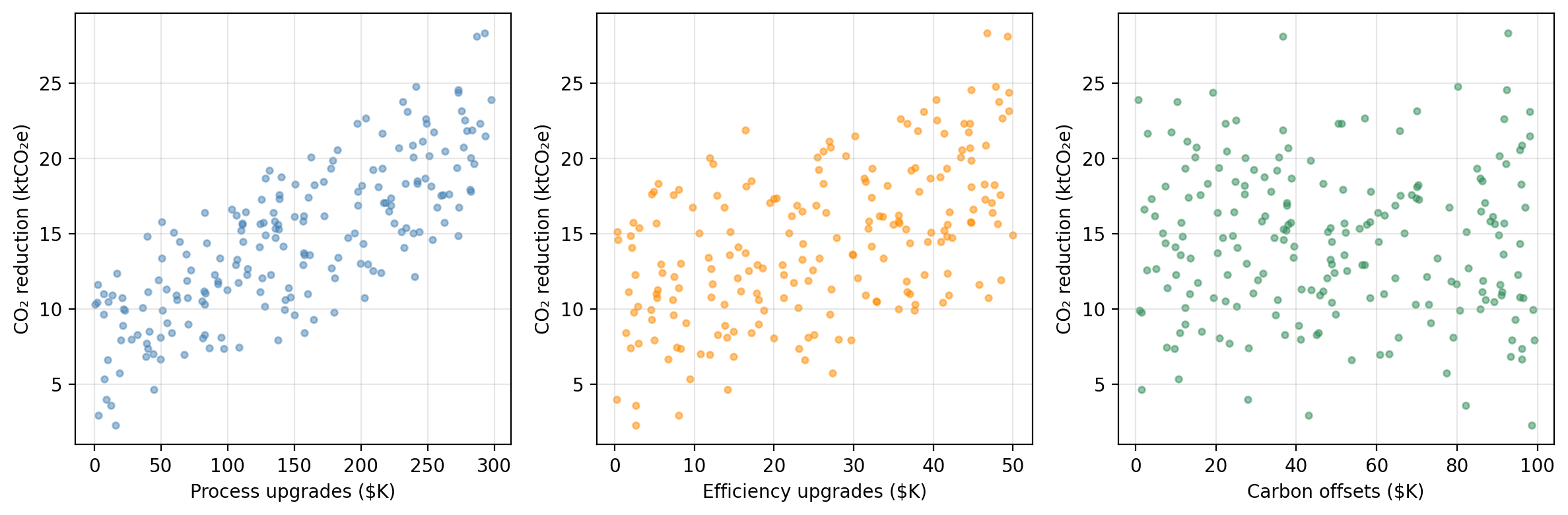
CO₂ reduction vs. each predictor
Synthetic data generated for educational purposes only
process spending: strongest linear association with CO₂ reductions. We will use this predictor as our variable today and go back to the others in the next lesson.
The simple linear regression model
Simple linear regression (SLR) assumes a linear relationship between a single predictor \(X\) and a response \(Y\):
\[Y \approx \beta_0 + \beta_1 X\]
- \(\beta_0 =\) \(y\)-intercept: expected value of \(Y\) when \(X = 0\)
- \(\beta_1 =\) slope: average change in \(Y\) for a one-unit increase in \(X\)
Since \(\beta_0\) and \(\beta_1\) are unknown, we estimate them from data:
\[\hat{y} = \hat{\beta}_0 + \hat{\beta}_1 x = \hat{f}(x)\]
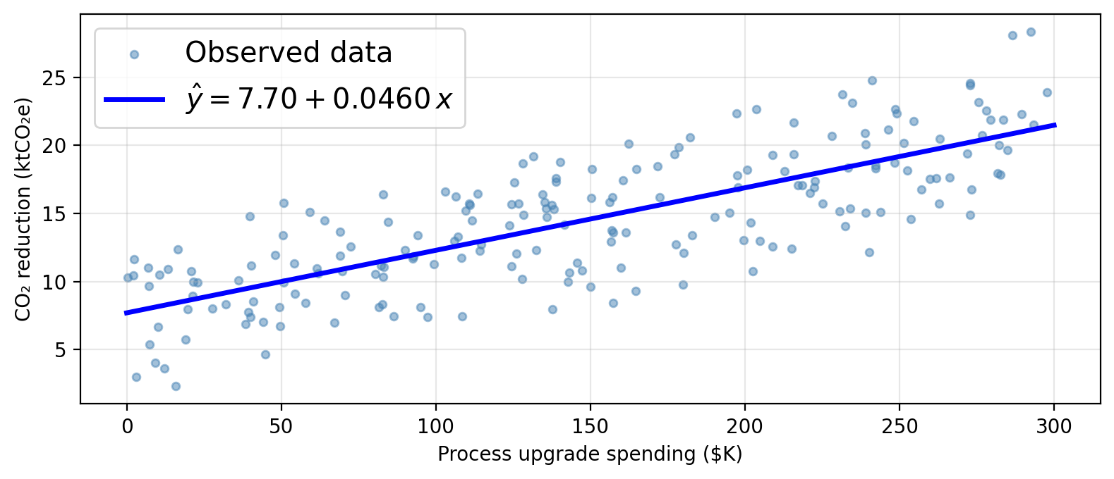
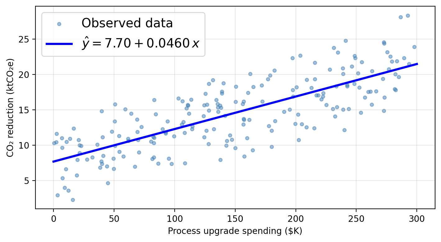
Using a linear model for our data
Using process as the sole predictor, a linear model for our data would assume this functional form:
\[\texttt{co2_reduction} \approx \hat{\beta}_0 + \hat{\beta}_1 \cdot \texttt{process}\]
Check-in
- How would you interpret the value of \(\hat{\beta}_0\)?
- How would you interpret the value of \(\hat{\beta}_1\)?
- If a firm spends $150K on process upgrades, how would you calculate the predicted CO₂ reduction?
Check-in
- How would you interpret the value of \(\hat{\beta}_0\)?
- How would you interpret the value of \(\hat{\beta}_1\)?
- If a firm spends $150K on process upgrades, how would you calculate the predicted CO₂ reduction?
\(\hat{\beta}_0 \approx\) 7.70 ktCO₂e: predicted CO₂ reduction when a firm spends $0 on process upgrades (baseline).
\(\hat{\beta}_1 \approx\) 0.0460 ktCO₂e per $K: each additional $1K in process spending is associated with 0.0460 ktCO₂e of additional reduction.
Just plug in 150 into the line equation!
Estimating the coefficients
Residuals and the RSS
Given \(n\) training observations \((x_1, y_1), \ldots, (x_n, y_n)\), we want to find \(\hat{\beta}_0\) and \(\hat{\beta}_1\) such that the line \(\hat{y} = \hat{\beta}_0 + \hat{\beta}_1 x\) is as close as possible to the observed data.
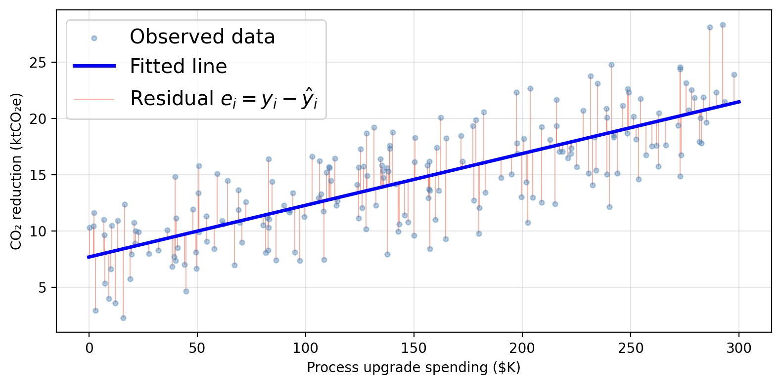
The residual for observation \(i\) is the difference between observed and predicted:
\[e_i = y_i - \hat{y}_i = y_i - \hat{\beta}_0 - \hat{\beta}_1 x_i\]
The residual sum of squares (RSS) totals all squared residuals:
\[RSS = \sum_{i=1}^{n} (y_i - \hat{y}_i)^2 = \sum_{i=1}^{n} (y_i - \hat{\beta}_0 - \hat{\beta}_1 x_i)^2.\]
The least squares approach to fit the regression line chooses \(\hat{\beta}_0\) and \(\hat{\beta}_1\) to minimize the RSS.
Residuals can be visualized as the vertical distance to the fitted line
Accuracy of the coefficient estimates
Standard errors
Our true function describing the relationship between predictor and response is given by \(f(X) = \beta_0 + \beta_1 X\). Our observed data is described by:
\[Y = f(X) + \epsilon = \beta_0 + \beta_1 X + \epsilon,\]
The standard error quantifies how far \(\hat{\beta}_i\) is from the true \(\beta_i\) on average.
The standard error for the slope \(\hat{\beta}_1\) is:
\[SE(\hat{\beta}_1)^2 = \frac{\sigma^2}{\sum_{i=1}^{n}(x_i - \bar{x})^2}\]
The standard error of the \(y\)-intercept \(\hat{\beta}_0\) is:
\[SE(\hat{\beta}_0)^2 = \sigma^2 \left[\frac{1}{n} + \frac{\bar{x}^2}{\sum_{i=1}^{n}(x_i - \bar{x})^2}\right]\]
\(\sigma^2 = \text{Var}(\epsilon)\) is the error variance (unknown in practice — estimated from the data).
Check-in: In these formulas, what do \(n\), \(x_i\), \(\bar{x}\) represent?
Confidence intervals
Standard errors allow us to construct confidence intervals for the true coefficients.
A 95% confidence interval is a range of values such that, if we repeated our experiment many times, approximately 95% of the computed intervals would contain the true parameter value.
A 95% confidence interval for a coefficient \(\beta_i\) is:
\[[\hat{\beta}_i - 2 \cdot SE(\hat{\beta}_i),\;\; \hat{\beta}_i + 2 \cdot SE(\hat{\beta}_i)]\]
(the factor 2 is approximate, the exact value comes from the \(t\)-distribution with \(n-2\) degrees of freedom)
Interpretation:
a 95% CI for \(\beta_1\) of \([a_1, b_1]\) means that, using a procedure that captures the true slope 95% of the time, we estimate that a one-unit increase of \(x\) is associated with an average increase in \(y\) between \(a_1\) and \(b_1\) units.
a 95% confidence inerval for \(\beta_0\) is \([a_0, b_0]\) means that, using a procedure that captures the true intercept 95% of the time, we estimate the model’s \(y\)-intercept is between \(a_0\) and \(b_0\).
Check-in
The exact 95% confidence intervals for each coefficient are:
95% CI for β₀ (intercept): [6.823, 8.567]
95% CI for β₁ (process):   [0.041, 0.051]
- What does the CI [0.041, 0.051] tell us about the relationship between process upgrade spending and CO₂ reductions?
- What if the interval had been [-0.002, 0.051] instead?
Interpretation:
Each additional $1K in process spending is associated with a reduction of between 0.041 and 0.051 ktCO₂e per year on average.
Also, the entire interval [0.041, 0.051] is above 0 so our procedure points to a positive slope: firms that invest more in cleaner production processes achieve greater CO₂ reductions.
An interval of [-0.002, 0.051] includes 0. We cannot rule out that \(\beta_1 = 0\), meaning we cannot confidently conclude that process spending drives reductions. Wider intervals generally arise from smaller samples or noisier data.
Is there a relationship between \(X\) and \(Y\)?
- Null hypothesis \(H_0\): no relationship between \(X\) and \(Y\).
In mathematical terms this means \(\beta_1 = 0\):
\[\hat{Y} = \hat{\beta}_0.\]
- Alternative hypothesis \(H_a\): there is some relationship between \(X\) and \(Y\).
In mathematical terms this means \(\beta_1 \neq 0\):
\[\hat{Y} = \hat{\beta}_0 + \hat{\beta}_1 X.\]
To test \(H_0\), we need to determine whether \(\hat{\beta}_1\) is sufficiently far from 0 relative to its uncertainty.
The \(t\)-statistic and \(p\)-value
The \(t\)-statistic measures how many standard deviations \(\hat{\beta}_1\) is from 0:
\[t = \frac{\hat{\beta}_1}{SE(\hat{\beta}_1)}.\]
If there truly is no relationship between the variables (\(\beta_1 = 0\)), then \(t\) follows a \(t\)-distribution with \(n - 2\) degrees of freedom.
The \(p\)-value is the probability of obtaining a \(t\)-statistic at least as large as the observed \(|t|\) in absolute value, assuming \(H_0\) is true.
\[
\begin{aligned}
&\text{Small } p\text{-value } (p < 0.05) \\
&\Rightarrow \text{unlikely to observe } |\hat{\beta}_1| \\
&\quad\text{this far from 0 by chance if } H_0 \text{ were true} \\
&\Rightarrow \textbf{reject } H_0 \\
&\Rightarrow \text{most likely } \beta_1 \neq 0 \\
&\Rightarrow \text{evidence of a relationship}\\
&\quad\text{between } X \text{ and } Y
\end{aligned}
\]
\[
\begin{aligned}
&\text{Large } p\text{-value} \\
&\Rightarrow \text{plausible to observe } |\hat{\beta}_1| \\
&\quad\text{this far from 0 by chance if } H_0 \text{ were true} \\
&\Rightarrow \textbf{fail to reject } H_0 \\
&\Rightarrow \beta_1 = 0 \text{ is consistent with the data} \\
&\Rightarrow \text{no evidence of a relationship}\\
&\quad\text{between } X \text{ and } Y
\end{aligned}
\]
Check-in
The table below shows the regression output for the SLR of co2_reduction on process:
          Coefficient Std. error t-statistic  p-value
Intercept      7.6953     0.4421       17.41 < 0.0001
  process      0.0460     0.0026       17.64 < 0.0001
- What does the \(p\)-value for
process tell us about the relationship between process upgrade spending and CO₂ reductions?
- The intercept also has a very small \(p\)-value. What does this mean about the intercept estimate? What would be an equivalent \(H_0\) for \(\beta_0\)?
- How would you interpret the coefficient for
process in plain language?
small \(p\)-value \(\Rightarrow\) strong evidence that \(\beta_1 \neq 0\): there is evidence of a positive relationship between process upgrade investment and CO₂ emissions reductions.
The \(p\)-value for the intercept tests \(H_0: \beta_0 = 0\). A small \(p\)-value means the regression line does not pass through the origin. There is likely some baseline CO₂ reduction even at zero process spending.
On average, each additional $1K invested in production processes is associated with ~0.046 ktCO₂e (46 metric tons) of additional CO₂ reduction.
\(R^2\) statistic
\(R^2\) measures the proportion of variance in \(Y\) explained by the model.
To compute it we need these ingredients:
- \(TSS = \sum_{i=1}^{n}(y_i - \bar{y})^2 =\) Total Sum of Squares: how much do the observations vary from the mean \(\bar{y}\): a way of measuring total variability in \(Y\)
- Intuitively: \(y_i = \hat{y}_i\) means a \(y\)-value is explained by the regression
- \(RSS = \sum_{i=1}^{n}(y_i - \hat{y}_i)^2 =\) Residual Sum of Squares: variability in \(y\) unexplained by the regression.
So
\[\underbrace{TSS}_{\text{total variability in }Y} - \underbrace{RSS}_{\text{unexplained by regression}} = \text{variability explained by regression}\]
We use this to define \[R^2 = \frac{TSS - RSS}{TSS}.\]
Interpreting \(R^2\)
\(R^2 \in [0, 1]\) always
\(R^2\) close to 1 → model explains most of the variability → good fit
\(R^2\) close to 0 → \(X\) alone is not capturing what drives \(Y\)
- Could mean: non-linear relationship, more predictors needed, high irreducible noise
Always look at your data: a high \(R^2\) does not guarantee a good model and a low \(R^2\) does not mean no relationship!
Check-in
For our SLR model of co2_reduction on process, we have that \(R^2\) = 0.611.
How would you interpret the \(R^2\) value in plain language?
An \(R^2\) of 0.611 means that approximately 61.1% of the variability in CO₂ reductions across firms is explained by a linear variation in process upgrade spending alone. The remaining ~38.9% of variability is driven by other factors not included in this model.
Residual Standard Error (RSE)
The RSE estimates the average amount the response deviates from the true regression line:
\[RSE = \sqrt{\frac{1}{n-2} RSS} = \sqrt{\frac{1}{n-2} \sum_{i=1}^{n}(y_i - \hat{y}_i)^2}\]
- A smaller RSE means predictions are closer to observed values
- RSE is in the same units as \(Y\) → directly interpretable
- “Small” is context-dependent: compare relative to the range or mean of \(Y\)
\(RSE\) and \(R^2\) are in-sample metrics
The \(R^2\) and \(RSE\) are computed on the same data used to fit the model.
These are in-sample measures, analogous to the training MSE from the previous lesson.
Remember:
- In-sample measures can give an overly optimistic picture of how the model generalizes to new data.
- For inference goals: use all available data to understand relationships between the variables
- For prediction goals: hold out a test set, fit on training data only, evaluate test MSE on the held-out set.
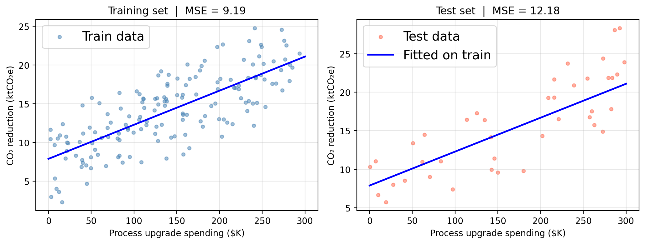
Train/test MSE for our SLR
SLR in the bias-variance framework
SLR has only 2 parameters (\(\hat{\beta}_0\), \(\hat{\beta}_1\)). It is a very rigid model:
Low variance: the fitted line generally changes little across different training samples drawn from the same population
Potentially high bias: if the true \(f\) is non-linear, a straight line will be systematically wrong regardless of how much data we collect
Inference vs. prediction
Inference
Goal: understand the relationship
Use all available data
Report \(R^2\), RSE, CIs, \(p\)-values
Example: “Does process spending drive CO₂ reductions?”
Prediction
Goal: forecast accurately for new observations
Hold out a test set
Report test MSE
Example: “Given spending levels, predict a firm’s CO₂ reduction”
In this lesson we covered
- Standard linear regression model: \(Y \approx \beta_0 + \beta_1 X\), estimated as \(\hat{Y} = \hat{\beta}_0 + \hat{\beta}_1 x\)
- Minimizing \(RSS = \sum(y_i - \hat{y}_i)^2\) gives us coeffient estimates \(\hat{\beta}_0, \hat{\beta}_1\)
- Standard errors quantify uncertainty in the coefficient estimates
- Confidence intervals give us a high-confidence method to estimate the coefficients
- We can use Hypothesis testing to figure out if there is a relationship between the variables
- \(p\)-value: probability of observing results if there was no variable relation \((H_0)\)
- small \(p\)-value → reject \(H_0\) → evidence of relation
- \(R^2\): proportion of variance in \(Y\) explained by the model