EDS 232 - Machine Learning for Environmental Science – multiple_linear

EDS 232

Lesson 4

Multiple linear regression

In this lesson

The multiple linear regression (MLR) model
Comparing MLR to individual SLRs
Hypothesis testing and the $F$-statistic
Model fit: $R^2$ in MLR and adjusted $R^2$
Variable selection: forward, backward, and mixed

A guiding example

Our example dataset

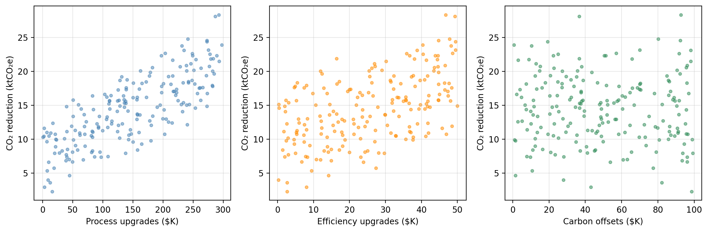
A research consortium tracks 200 manufacturing firms. For each firm, they record annual spending on three emissions-reduction strategies and the resulting CO₂ savings:

process — investment in cleaner production processes ($K/year)
efficiency — investment in energy efficiency upgrades ($K/year)
offsets — carbon offset purchases ($K/year)
co2_reduction — annual CO₂ emissions reduced (ktCO₂e/year)

The researchers want to understand:

Do these investments actually drive emissions reductions, and if so, by how much?

CO₂ reduction vs. each predictor

Synthetic data generated for educational purposes only

From SLR to MLR

In SLR we modelled the relationship between one predictor and a response:

\[\texttt{co2_reduction} \approx \hat{\beta}_0 + \hat{\beta}_1 \cdot \texttt{process}.\]

Our example dataset has three potential predictors.

Running separate SLRs has the problem that each SLR ignores the other predictors.

Multiple linear regression handles all predictors simultaneously.

The multiple linear regression model

The MLR model

With $p$ predictors $X_1, \ldots, X_p$ and response variable $Y$, the multiple linear regression (MLR) model assumes the predictors and response are related by:

\[Y = \beta_0 + \beta_1 X_1 + \beta_2 X_2 + \cdots + \beta_p X_p + \epsilon,\]

each $\beta_i$ is a coefficient and $\epsilon$ is an error term.

In our example data

$Y =$ co2_reduction is the response variable
$p = 3$ is the number of predictors

$X_1 =$ process is predictor 1
$X_2 =$ efficiency is predictor 2
$X_3 =$ offset is predictor 3

So the MLR model takes the form:

\[\texttt{co2_reduction} = \beta_0 + \beta_1 \cdot \texttt{process} + \beta_2 \cdot \texttt{efficiency} + \beta_3 \cdot \texttt{offsets} + \epsilon.\]

Estimating the MLR coefficients

In the MLR model we assume: $Y = \beta_0 + \beta_1 X_1 + \beta_2 X_2 + \cdots + \beta_p X_p + \epsilon.$

Our goal is to estimate the coefficients and obtain a model

\[\hat{Y} = \hat{\beta}_0 + \hat{\beta}_1 X_1 + \hat{\beta}_2 X_2 + \cdots + \hat{\beta}_p X_p.\]

Our training set is $\{(x_1, y_1), \ldots, (x_n, y_n)\}$ with $n$ observations.

For each of the observations $(x_i, y_i)$ we have that:

$x_i = (x_{i1}, x_{i2}, \ldots, x_{ip})$ is a vector of $p$ predictor values, and
$y_i$ is the response associated to $x_i$.

We estimate the coefficients/fit the model by finding the $\hat{\beta}_i$ that minimize the residual sum of squares (same procedure as SLR!):

\[ RSS = \sum_{i=1}^{n} (y_i - \hat{y}_i)^2 = \sum_{i=1}^{n} (y_i - \hat{\beta}_0 - \hat{\beta}_1x_{i1} - \ldots - \hat{\beta}_px_{ip})^2 . \]

Interpreting the MLR coefficients

Once we find the coefficients that minimize the RSS we obtain a model:

\[\hat{Y} = \hat{\beta}_0 + \hat{\beta}_1 X_1 + \hat{\beta}_2 X_2 + \cdots + \hat{\beta}_p X_p\]

We interpret each coefficient as

$\hat{\beta}_j$ is the average change in $Y$ associated with a one-unit increase in $X_j$, holding all other predictors constant.

Check-in

For our example data, the estimated coefficients are:

           MLR coeff
 intercept    3.4543
   process    0.0461
efficiency    0.1831
   offsets   -0.0088

And we obtain the model: \[\text{co2_reduction} = 3.4543 + 0.0461*\text{process} + 0.1831*\text{efficiency} -0.0088*\text{offsets}\]

What is the interpretation of the efficiency coefficient of 0.1831?
How do we calculate the predicted CO₂ reduction for a firm that spends $100K on process upgrades, $20K on efficiency, and $50K on offsets?
The offsets coefficient is very small and negative. What does that mean?

Check-in

For our example data, the estimated coefficients are:

           MLR coeff
 intercept    3.4543
   process    0.0461
efficiency    0.1831
   offsets   -0.0088

And we obtain the model: \[\text{co2_reduction} = 3.4543 + 0.0461*\text{process} + 0.1831*\text{efficiency} -0.0088*\text{offsets}\]

What is the interpretation of the efficiency coefficient of 0.1831?
How do we calculate the predicted CO₂ reduction for a firm that spends $100K on process upgrades, $20K on efficiency, and $50K on offsets?
The offsets coefficient is very small and negative. What does that mean?

Each additional $1K in energy efficiency upgrades is associated with 0.1831 ktCO₂e of additional CO₂ reduction, holding process and offset spending constant.
Using our model, the estimate is given by $\hat{y} = \hat{\beta}_0 + \hat{\beta}_1 \cdot 100 + \hat{\beta}_2 \cdot 20 + \hat{\beta}_3 \cdot 50 \approx 11.29$ ktCO₂e.
It means if we hold process and efficiency spending constant, higher offset purchases are associated with a slightly lower CO₂ reduction.

Accuracy of the coefficient estimates

Information about standard errors and confidence intervals for the MLR coefficients.

$p$-values for the coefficients

In SLR, the $p$-value for $\hat{\beta}_1$ tests $H_0: \beta_1 = 0$, which means is $X$ related to $Y$?

In MLR, the $p$-value for each $\hat{\beta}_j$ tests $H_0: \beta_i =0$, which means is $X_i$ related to $Y$ if all other predictor are in the model?

So $H_0$ for MLR is about the partial effect of $X_j$. We are trying to answer:

Does $X_j$ add information beyond what the other predictors already explain?

We can interpret the individual $p$-values from the MLR as

Small $p$-value for $\hat{\beta}_j$ → $X_j$ is informative given the other predictors are in the model
Large $p$-value for $\hat{\beta}_j$ → $X_j$ adds little beyond what the others already capture

Check-in

For our example data we obtaing the following estimates and $p$-values for the coefficients associated with the predictors

 Predictor MLR coeff MLR p-value
   process    0.0461    < 0.0001
efficiency    0.1831    < 0.0001
   offsets   -0.0088      0.0193

How can we interpret the $p$-value associated with the process variable?
Suppose your $p$-value threshold is 0.01. What does the offsets $p$-value tell us in the context of this MLR model?

Check-in

For our example data we obtaing the following estimates and $p$-values for the coefficients associated with the predictors

 Predictor MLR coeff MLR p-value
   process    0.0461    < 0.0001
efficiency    0.1831    < 0.0001
   offsets   -0.0088      0.0193

How can we interpret the $p$-value associated with the process variable?
Suppose your $p$-value threshold is 0.01. What does the offsets $p$-value tell us in the context of this MLR model?

There is a relationship between the process predictor and the response variable co2_reduction, when the efficiency and offsets remain fixed.
It is detecting that offset spending contributes almost nothing beyond what process and efficiency already capture.

Comparing MLR to individual SLRs

SLR vs. MLR: why not just run $p$ separate regressions?

individual SLR coefficients can be misleading when predictors are correlated
When two predictors are correlated, each one’s SLR coefficient absorbs part of the other’s effect.

Example

Suppose firms that invest heavily in process upgrades tend to also invest heavily in efficiency.

An SLR of co2_reduction on process alone will give a coefficient that also reflects some of the efficiency effect.
The MLR coefficient for process strips out the efficiency effect and reflects only the direct relationship of process.

SLR vs. MLR: why not just run $p$ separate regressions?

individual SLR coefficients can be misleading when predictors are correlated
When two predictors are correlated, each one’s SLR coefficient absorbs part of the other’s effect.

Example

In our example dataset, SLR ≈ MLR coefficients because the predictors were drawn independently (uncorrelated by construction).

 Predictor SLR coeff SLR p-value MLR coeff MLR p-value
   process    0.0460    < 0.0001    0.0461    < 0.0001
efficiency    0.1793    < 0.0001    0.1831    < 0.0001
   offsets   -0.0060      0.6153   -0.0088      0.0193

In real data, predictors can be correlated. The divergence between SLR and MLR coefficients can be large.
The MLR coefficient reflects the direct effect of each predictor, holding the others constant.

Hypothesis testing & the F-statistic

Is any predictor related to the response?

In SLR: $Y \approx \beta_0 + \beta_1 X$ and we tested

$H_0$: $\beta_1=0 \Rightarrow$ no relationship between response and predictor
$H_a$: $\beta_1\neq0 \Rightarrow$ some relationship between response and predictor.

For MLR: $Y \approx \beta_0 + \beta_1X_1 + \ldots + \beta_p X_p$ and we can test

$H_0$: $\beta_1 =... =\beta_p=0 \Rightarrow$ no relationship between $Y$ and any predictor $X_1, \ldots, X_p$
$H_a$: at least one $\beta_j \neq 0 \Rightarrow$ some relationship between response and some predictor.

We are investigating the question Is any predictor related to the response?

The F-statistic

We are investigating the question Is any predictor related to the response?

We test this with the $F$-statistic:

\[F = \frac{(TSS - RSS)/p}{RSS/(n - p - 1)}\]

$TSS = \sum(y_i - \bar{y})^2$ is the total variability in $Y$,
$RSS = \sum(y_i - \hat{y}_i)^2$ is the variability unexplained by the model,

Numerator: how much variance the predictors collectively explain
Denominator: how much variance remains unexplained per degree of freedom

$F \approx 1$: no predictor is related to $Y$ → consistent with $H_0$
$F \gg 1$: at least one predictor explains variance beyond noise → evidence against $H_0$

An associated $p$-value is then computed to assess the probability of observing an $F$-statistic this large or larger, assuming $H_0$ is true.

Example

   Quantity    Value
F-statistic   612.13
    p-value < 0.0001

An $F$-statistic of 612.1 with $p \ll 0.05$ gives very strong evidence that at least one predictor is associated with CO₂ reductions.

Check-in

Pair up with someone. Have one person explain the hypothesis test for simple linear regression and the other explain the hypothesis test for multiple linear regression.

Hypothesis testing steps

From EDS 222.

Identify the TEST STATISTIC
State your NULL and ALTERNATIVE hypotheses
Calculate the OBSERVED test statistic
Estimate the NULL DISTRIBUTION
Calculate P-VALUE
Compare p-value to CRITICAL THRESHOLD

Why not just use individual p-values?

Earlier we saw that each coefficient of the MLR has an associated $p$-value. So one my ask: why do we need a $p$-value for the $F$-statistic, when we can just interpet each $p$-value individually?

For an individual coefficient, a $p$-value of 0.05 means:

“if there is truly no relationship ($H_0$ true), there is a 5% probability of getting a $t$-statistic this extreme just by random chance.”

Suppose $p=100$ and there’s truly no association between any predictor and the response. We would expect about 5% of our $t$-statistics to be “false positives” just by random chance.

When $p$ is large, we run the risk of some individual $p$-values being small by chance even when no predictor is truly related to $Y$.

The $F$-statistic tests all coefficients jointly and accounts for this.

Model fit: R² and adjusted R²

$R^2$ in multiple regression

The $R^2$ formula is the same as in SLR:

\[R^2 = 1 - \frac{RSS}{TSS}\]

It measures the proportion of variance in $Y$ explained by the model.

Important: adding a predictor to an MLR model will increase $R^2$ or leave it unchanged, even if that predictor has no real relationship with $Y$.

The adjusted $R^2$ penalizes for the number of predictors:

\[\bar{R}^2 = 1 - \frac{RSS/(n-p-1)}{TSS/(n-1)}\]

Adjusted $R^2$ can decrease when an irrelevant predictor is added. Better for comparing models of different sizes.

Check-in

                     Model    R² Adj. R²
        SLR (process only) 0.611   0.609
MLR (all three predictors) 0.904   0.902

$R^2$ increased when going from SLR to MLR. Does this mean the MLR is a better model?
The adjusted $R^2$ also increased. What does this tell us?

Probably, but remember $R^2$ always increases (or stays flat) when predictors are added, even useless ones. It cannot be used alone to compare models of different sizes.
Adjusted $R^2$ penalizes for each extra predictor. The fact that it also increased means efficiency (and possibly offsets) are contributing enough to justify their inclusion.

Variable selection

Which predictors should we include?

With $p$ predictors there are $2^p$ possible ways of choosing which predictors to use:

$p = 3$: 8 models — feasible to compare exhaustively
$p = 10$: 1,024 models
$p = 30$: over 1 billion models — completely infeasible

Three common automated approaches for large $p$:

Forward selection: start with nothing, add one predictor at a time
Backward selection: start with everything, remove one at a time
Mixed selection: combine forward and backward steps

Forward and backward selection

Forward selection

Start: null model (intercept only)
Add the predictor with the largest RSS reduction
Repeat until some stopping criterion is met

✓ Always applicable

✗ A variable added early may become redundant later

Can be run using other metrics instead of RSS (ex: adjusted $R^2$)

Forward and backward selection

Forward selection

Start: null model (intercept only)
Add the predictor with the largest RSS reduction
Repeat until some stopping criterion is met

✓ Always applicable

✗ A variable added early may become redundant later

Can be run using other metrics instead of RSS (ex: adjusted $R^2$)

Backward selection

Start: full model (all $p$ predictors)
Remove the predictor with the largest $p$-value
Repeat until all remaining predictors are significant

✓ Considers all predictors from the start

✗ Cannot be used when $p > n$

Can be run using other metrics instead of $p$-values (ex: adjusted $R^2$)

Check-in

                    Predictors    RSS
              (intercept only) 5016.8
                       process 1950.3
                    efficiency 3601.4
                       offsets 5010.4
          process + efficiency  497.5
             process + offsets 1949.8
          efficiency + offsets 3571.4
process + efficiency + offsets  483.8

Forward selection process

Start: null model (intercept only)
Add the predictor with the largest RSS reduction
Repeat until some stopping criterion is met

Trace through forward selection using this table.

Which predictor would be added first? Second? Does adding offsets meaningfully reduce RSS?
What criteria could be used to decide whether to add or not the final predictor?

Check-in

                    Predictors    RSS
              (intercept only) 5016.8
                       process 1950.3
                    efficiency 3601.4
                       offsets 5010.4
          process + efficiency  497.5
             process + offsets 1949.8
          efficiency + offsets 3571.4
process + efficiency + offsets  483.8

Forward selection process

Start: null model (intercept only)
Add the predictor with the largest RSS reduction
Repeat until some stopping criterion is met

Trace through forward selection using this table.

Which predictor would be added first? Second? Does adding offsets meaningfully reduce RSS?
What criteria could be used to decide whether to add or not the final predictor?

process is added 1st (lowest RSS)
efficiency is added 2nd: Substantial RSS reduction, efficiency spending is genuinely associated with CO₂ reductions.
Adding offsets to the two-predictor model produces only a very small reduction in RSS
A minimum RSS reduction at each step.

Check-in

Step 1 — full model

 Predictor  p-value
   process < 0.0001
efficiency < 0.0001
   offsets   0.0193

Step 2 — after first removal

 Predictor  p-value
   process < 0.0001
efficiency < 0.0001

Backward selection

Start: full model (all $p$ predictors)
Remove the predictor with the largest $p$-value
Repeat until all remaining predictors are significant

Using the $p$-value tables, trace through backward selection step by step.

Which predictor is removed first? Why?
Should we remove another predictor in step 2, or stop?

Check-in

Step 1 — full model

 Predictor  p-value
   process < 0.0001
efficiency < 0.0001
   offsets   0.0193

Step 2 — after first removal

 Predictor  p-value
   process < 0.0001
efficiency < 0.0001

Backward selection

Start: full model (all $p$ predictors)
Remove the predictor with the largest $p$-value
Repeat until all remaining predictors are significant

Step 1: offsets has by far the largest $p$-value → remove it
Step 2: both process and efficiency have very small $p$-values → all remaining predictors are significant; stop

Mixed selection

Mixed selection (stepwise) combines forward and backward steps:

Start with the null model
Forward step: add the variable with the largest RSS reduction
Backward step: check if any included variable now has a large $p$-value. If so, remove it
Continue until all variables in the model have sufficiently low $p$-value, and all variables outside the model would have a large $p$-value if added.

This fixes the main weakness of forward selection: a variable added early can be removed once other, better variables are in the model.

Variable selection: in practice

Use forward when:

$p$ is large or $p > n$: backward requires fitting the full model, which is impossible when there are more predictors than observations
You expect only a few predictors to matter

Use backward when:

$p$ is small and $n$ is large enough to fit the full model comfortably (the more common situation in environmental science)
You are worried about missing a predictor that only becomes significant in the presence of others — backward sees all predictors simultaneously from the start

In practice:

Mixed selection hedges against the weaknesses of both. Many practitioners run all three and check whether they agree
If all three disagree, that signals correlated predictors and no single “right” model

Modern practice often prefers regularization (lasso, ridge) over stepwise selection — these methods perform variable selection and coefficient estimation simultaneously and have better statistical properties. More on this later in the course.

In this lesson we covered

MLR model: $Y = \beta_0 + \beta_1 X_1 + \cdots + \beta_p X_p + \epsilon$ — coefficients interpreted holding all else constant
Least squares minimizes RSS
Individual p-values: test partial effects (does $X_j$ add beyond the others?)
F-statistic: tests $H_0: \beta_1 = \cdots = \beta_p = 0$
$R^2$ always increases with predictors; use adjusted $R^2$ to compare models of different sizes
Variable selection: forward, backward, mixed