EDS 232
Lesson 5
KNN and accuracy metrics
In this lesson
- The classification setting and how it differs from regression
- K-Nearest Neighbors (KNN) as a simple classification method
- Accuracy assessment: the confusion matrix, precision, recall, and \(F_1\) score
- Overfitting in classification and the bias-variance tradeoff
From regression to classification
From regression to classification
So far, our response variable \(Y\) has always been quantitative.
In many real-world problems the response is qualitative (categorical): meaning the response takes a value in a discrete set of classes.
Classifying = predicting the class of a new observation.
Classic examples:
- Is this email spam or not?
- Handwritten character recognition
- Image classification
Environmental examples:
- Does a water sample exceed a contamination threshold?
- Is a species present or absent at a given location?
- Is a certain study site healthy or degraded?
Our example dataset
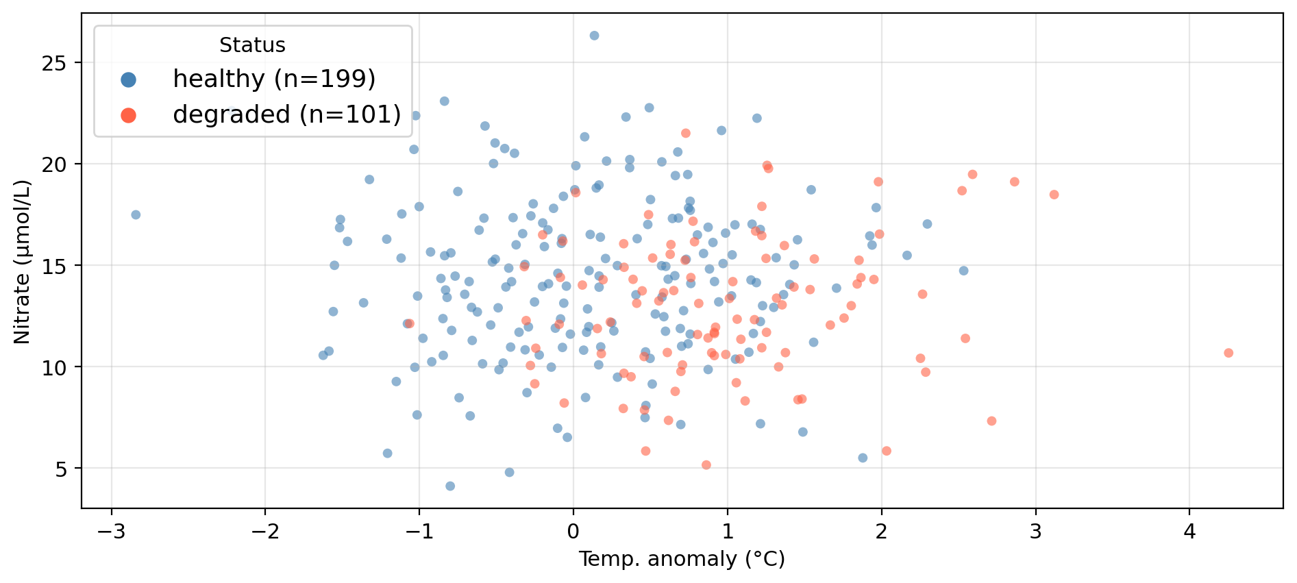
A synthetic dataset “tracking” 300 coastal monitoring stations along CA coast:
temp_anomaly — sea surface temperature anomaly (°C): deviation of ocean’s temperature from long-term averagenitrate — nitrate concentration (μmol/L)status — kelp forest condition: healthy or degraded
Can we predict whether a site is healthy or degraded
based on its oceanographic conditions?
Data overview
Synthetic data generated for educational purposes only
The KNN algorithm
- One of the simplest classification methods
- Classify a new observation by majority vote among its nearest neighbors in the training data
Given a training set and a new test observation \(x_0\):
- Choose an integer \(K \geq 1\).
- Identify the \(K\) points in the training data closest to \(x_0\).
- Identify the majority class among those \(K\) neighbors.
- Assign that class as the prediction for \(x_0\).
There is no model training or fitting.
Just store the data and vote at prediction time.
Check-in
KNN algorithm:
- Choose an integer \(K \geq 1\).
- Identify the \(K\) points in the training data closest to \(x_0\).
- Identify the majority class among those \(K\) neighbors.
- Assign that class as the prediction for \(x_0\).
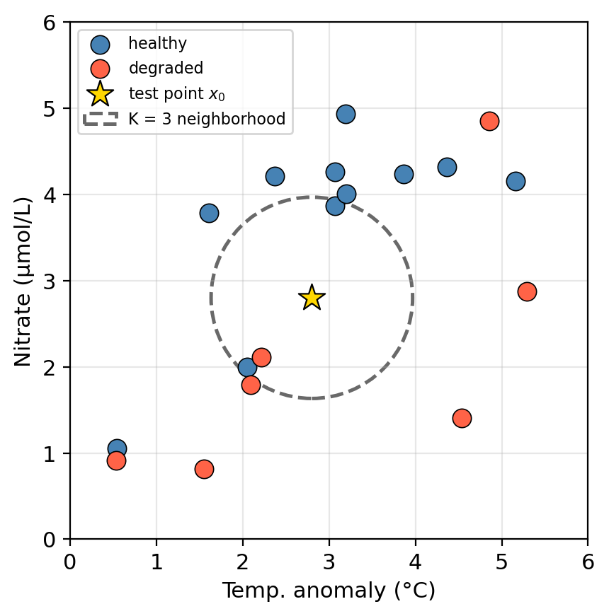
Using K=3:
- What class would KNN assign to \(x_0\)? Why?
- What would change if we used \(K=1\) instead?
- What would happen if \(K =\) total number of training observations?
Check-in
KNN algorithm:
- Choose an integer \(K \geq 1\).
- Identify the \(K\) points in the training data closest to \(x_0\).
- Identify the majority class among those \(K\) neighbors.
- Assign that class as the prediction for \(x_0\).
- Healthy. Two of the three neighbors are blue (healthy), so healthy wins the majority vote.
- With \(K=1\) the predictions are determined by the single closest training point.
- We would always predict the majority class for every observation.
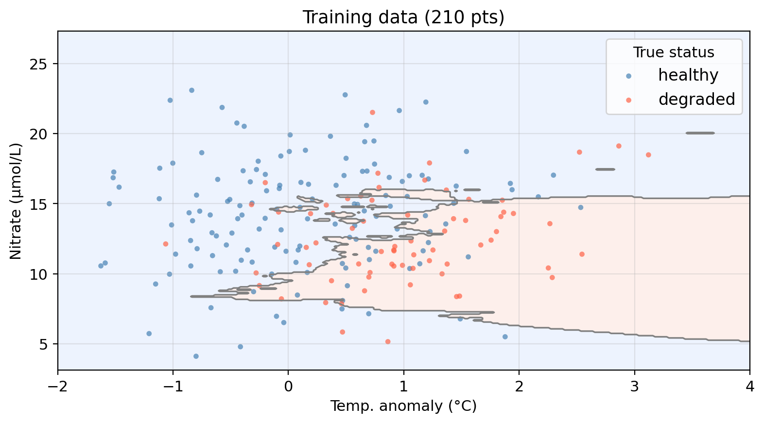
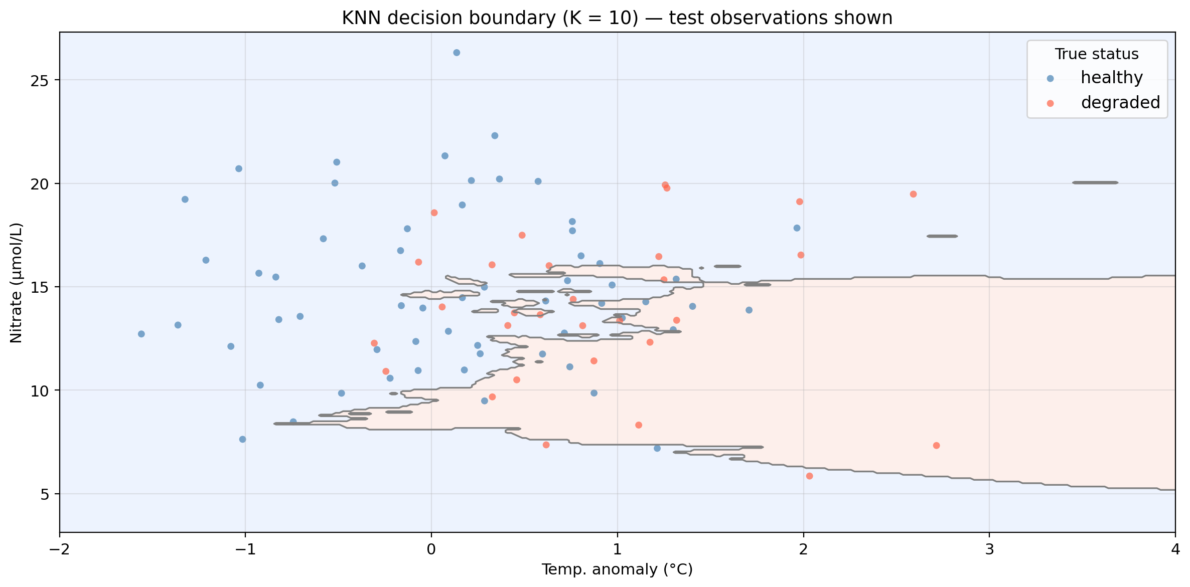
Applying KNN to example data (K = 10)
Shaded regions = predicted class. Decision boundary = boundary between predicted class regions.
Points in the “wrong” region are misclassified.
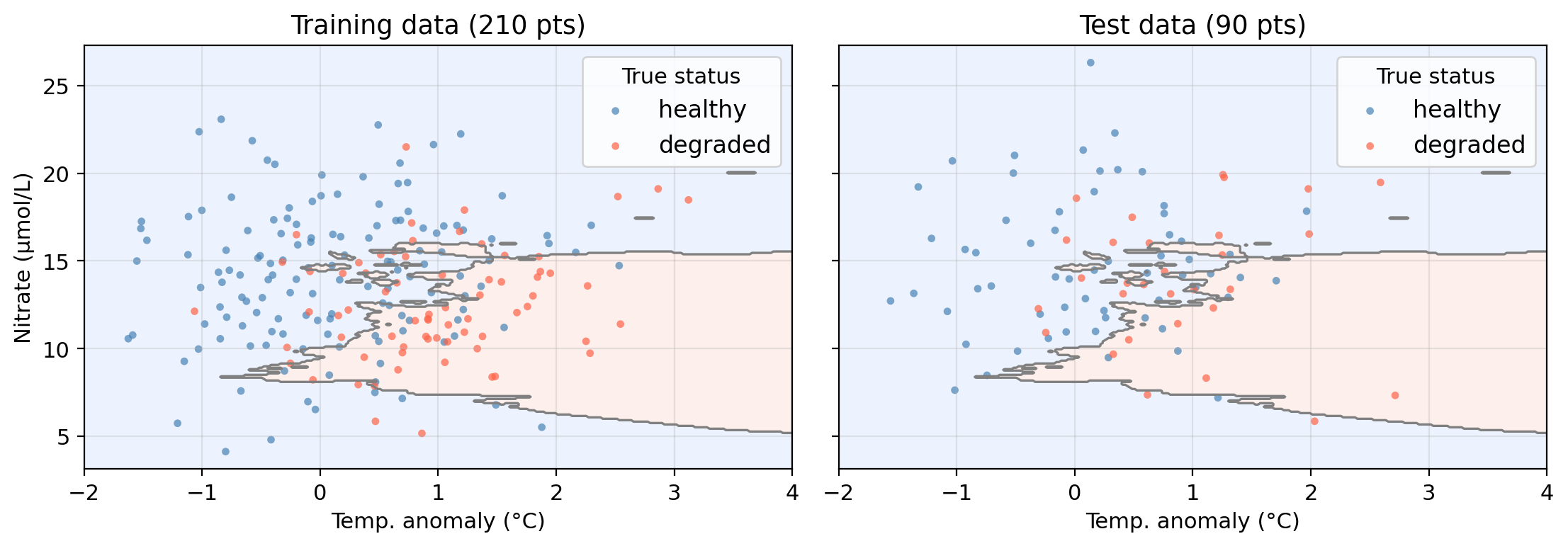
Applying KNN to example data (K = 10)
Shaded regions = predicted class. Decision boundary = boundary between predicted class regions.
Points in the “wrong” region are misclassified.
KNN: pros and cons
Pros
- Non-parametric: no assumptions about the model’s functional form
- Simple and intuitive: no explicit model to train
- Naturally handles multi-class problems
Cons
- Slow at prediction time: must compute distance to every training point
- Performance degrades as number of predictors grows
Other considerations
- Sensitive to predictor scale, standardization usually required
- Choice of \(K\) requires cross-validation (we will talk about this next week)
Accuracy assessment for classifiers
True and false positives and negatives
- Binary classifier: two classes, positive and negative.
- Each test observation falls into one of four categories:
| True Positive |
Positive |
Positive |
Yes |
| True Negative |
Negative |
Negative |
Yes |
| False Positive |
Negative |
Positive |
No |
| False Negative |
Positive |
Negative |
No |
Check-in
Using healthy = positive class, classify each observation as true positive, true negative, false positive, or false negative:
| A |
healthy |
healthy |
| B |
degraded |
healthy |
| C |
healthy |
degraded |
| D |
degraded |
degraded |
Check-in
Using healthy = positive class, classify each observation as true positive, true negative, false positive, or false negative:
| A |
healthy |
healthy |
| B |
degraded |
healthy |
| C |
healthy |
degraded |
| D |
degraded |
degraded |
- A → true positive
- B → false positive
- C → false negative
- D → true negative
Check-in
Identify one true positive point, one true negative point, one false positive point, and one false negative point.
The confusion matrix
To summarize the accuracy of our classifier we
- Predict the class for every point in our test set and compare it against its true class
- Count the number of true/false positives and true/false negatives we obtained:
- TP: correctly predicted positives
- TN: correctly predicted negatives
- FP: negative observations predicted as positive
- FN: positive observations predicted as negative
and arrange them in a confusion matrix:
| True class is positive |
TP |
FN |
| True class is negative |
FP |
TN |
The confusion matrix shows at a glance where the classifier makes mistakes and what kinds of errors it makes.
Accuracy metrics
Overall accuracy: fraction of correctly classified observations \[\text{accuracy} = \frac{TP + TN}{TP + FP + TN + FN}\]
Precision: of all the predicted positives, how many are truly positive? \[\text{precision} = \frac{TP}{TP + FP}\]
Recall (sensitivity): of all observations whose true class is positive, how many did we correctly identify? \[\text{recall} = \frac{TP}{TP + FN}\]
All metrics range from 0 (worst) to 1 (best).
Precision and recall trade off against each other:
- High recall → catch almost everything, but may have many false alarms
- High precision → predictions are reliable, but may miss many positives
The right balance depends on the cost of each error type.
Check-in
A classifier always predicts positive. What is its recall? What is its precision?
A classifier rarely predicts positve but, when it does, it is always correct. What would recall be like? And precision?
You are a conservation manager allocating resources to degraded sites. Would you prioritize precision or recall? Why?
Overall accuracy: fraction of correctly classified observations \[\text{accuracy} = \frac{TP + TN}{TP + FP + TN + FN}\]
Precision: of all the predicted positives, how many are truly positive? \[\text{precision} = \frac{TP}{TP + FP}\]
Recall (sensitivity): of all observations whose true class is positive, how many did we correctly identify? \[\text{recall} = \frac{TP}{TP + FN}\]
Check-in
A classifier always predicts positive. What is its recall? What is its precision?
A classifier rarely predicts positve but, when it does, it is always correct. What would recall be like? And precision?
You are a conservation manager allocating resources to degraded sites. Would you prioritize precision or recall? Why?
Recall = 1.0 (no true positive is ever missed). Precision is low: it predicts positive for every observation, including negatives.
High precision and low recall.
Likely recall since you want to catch as many truly degraded sites as possible. A missed degraded site (FN) means no intervention, which can have direct consequences.
The \(F_1\) score
One way of summarzing precision and recall into a single metric:
\[F_1 = \frac{2 \cdot \text{precision} \times \text{recall}}{\text{precision} + \text{recall}}\]
- Ranges from 0 (worst) to 1 (best)
- Favors classifiers with balanced precision and recall
- A model with high precision but very low recall (or vice versa) gets a low \(F_1\)
- Simple way to compare classifiers, but you should examine all metrics individually!
Check-in
The null classifier always predicts the majority class, ignoring all predictors. Any useful model should outperform it! The following table shows accuracy metrics for tne KNN (K=10) classifier and the null classifier:
          Model Accuracy Precision Recall F₁ score
Null classifier    0.667     0.667  1.000    0.800
   KNN (K = 10)    0.656     0.710  0.817    0.760
- The null classifier has recall = 1.000 but a lower \(F_1\). Why?
- Both models have similar overall accuracy. Is OA alone a good summary to assess whether KNN is no better than the null classifier?
The null always predicts healthy (positive), so it never misses a true positive → perfect recall. But it misclassifies every degraded site, bringing down precision and \(F_1\).
The two classifiers have similar accuracy, yet KNN has some evidence of distinguishing between classes rather than blindly predicting the majority.
Overfitting and the bias-variance tradeoff
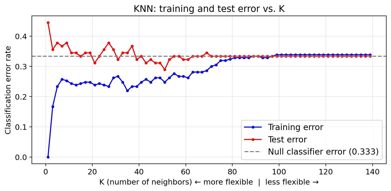
Classification error rate
Classification error rate
In classification we use the error rate as a simple measure of model performance:
\[\text{error rate} = \frac{\text{# misclassified observations}}{\text{total observations}} = \frac{FP + FN}{TP + FP + TN + FN}\]
We compute both a training error rate and a test error rate by calculating the error rate on the training and test sets (similarly to how we calcualted the MSE for regression problems).
As in regression, a model is overfitting when it has a small training error but a large test error.
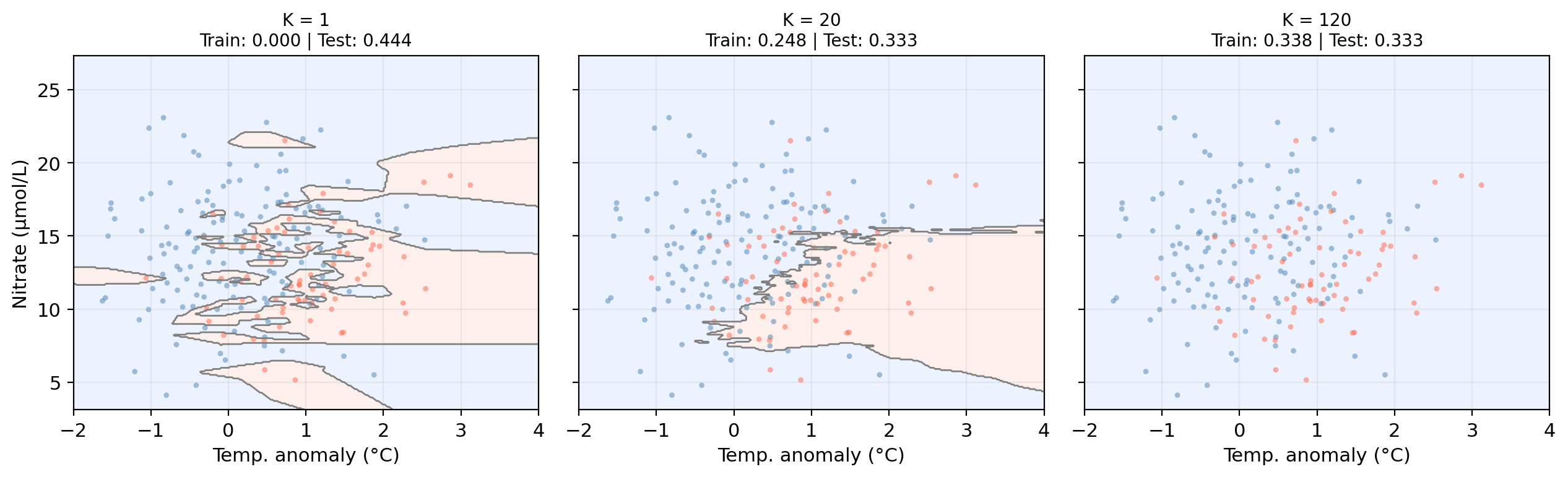
KNN boundaries for different K
Check-in
- At \(K = 1\), what is the training error? Why?
- Where is the classifier overfitting?
- Where would you choose \(K\) to get the best generalization performance?
Check-in
- Training error = 0. With K = 1, every point’s nearest neighbor is itself: always classified correctly.
- Left side (small K): training error is near zero but test error is noticeably higher. Gap indicates overfitting.
- Near where the error rate is minimized
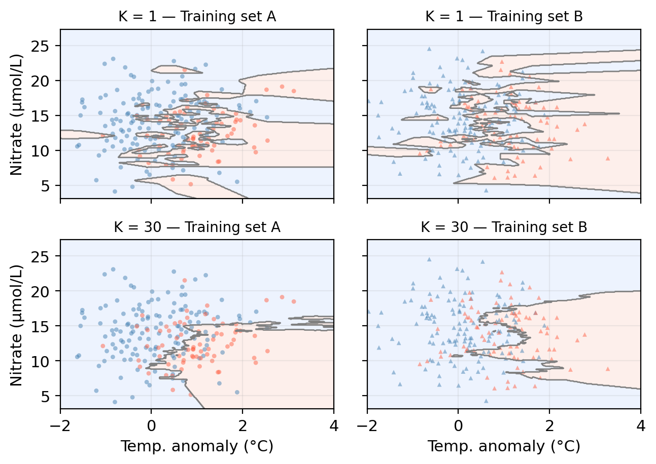
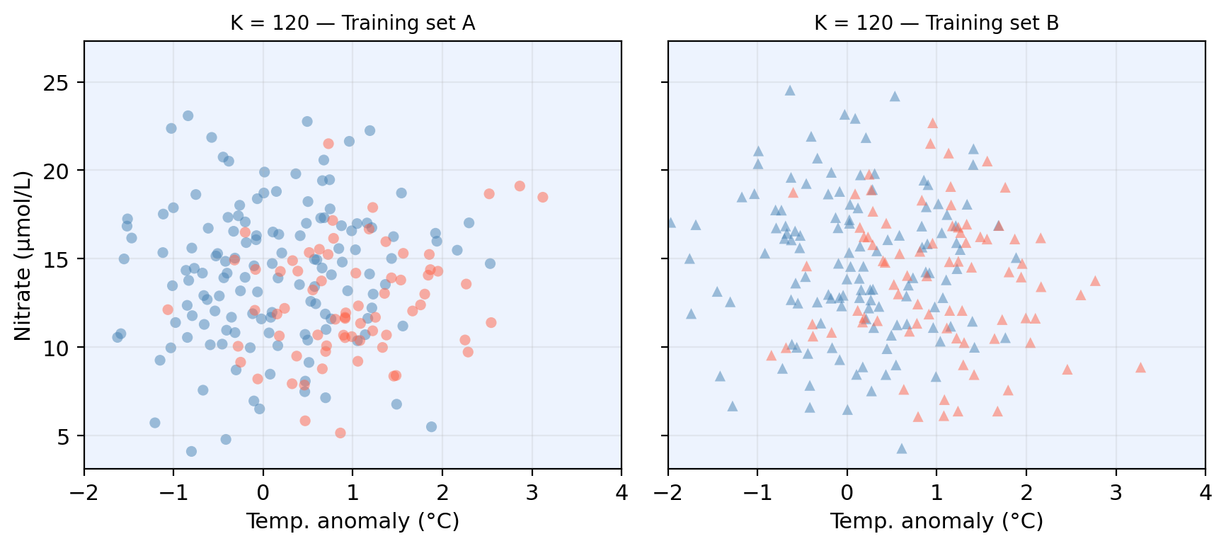
Model variance
Model variance: how much our model would change if trained on a different dataset.
Check-in: Whick \(K\) do you think gives a model with higher variance?
Model bias
Model bias refers to the error introduced by the assumptions built into the model. Models with high bias will be systematically wrong, no matter how much training data we give it.
What do you notice about the two boundaries? What does this tell us?
The bias-variance tradeoff: classification
High flexibility model often shows low bias and high variance.
- The flexible classification boundary can capture complex patterns but changes a lot from one training sample to another.
Low flexibility model often shows high bias and low variance.
- The rigid boundary is stable but may systematically miss real structure in the data.
In the case of KNN:
| Flexibility |
High |
Low |
| Bias |
Lower |
Higher |
| Variance |
Higher |
Lower |
Test error is minimized at an intermediate K that balances bias and variance.