EDS 232
Lesson 6
Logistic regression and ROC curves
In this lesson
- Logistic regression and how it is used for classification
- Interpreting logistic regression coefficients through log-odds
- Adjusting the classification threshold and its effect on precision and recall
- ROC curves and the AUC as tools for evaluating classifier performance across thresholds
Our example dataset
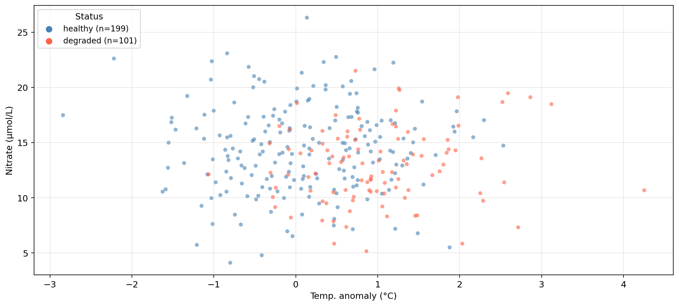
The same synthetic dataset from the previous lesson — 300 coastal monitoring stations:
temp_anomaly — sea surface temperature anomaly (°C): deviation from long-term averagenitrate — nitrate concentration (μmol/L)status — kelp forest condition: healthy or degraded
Can we predict whether a site is healthy or degraded
based on its oceanographic conditions?
Data overview
Synthetic data generated for educational purposes only
Logistic regression
Rather than predicting the class directly, logistic regression models the probability that an observation belongs to the positive class:
\[P(Y = 1 \mid X) = p(X).\]
Once we have \(p(X)\), we classify \(X\) using a classification threshold \(\alpha\):
\[
\text{the class of $X$ is} = \begin{cases} \text{class } 1, & \text{if } p(X) \geq \alpha \\ \text{class } 0, & \text{if } p(X) < \alpha \end{cases}.
\]
The choice of threshold is something we control.
Logistic regression: example data
Logistic regression: example data
In our example:
- Predictor:
temp_anomaly
- Response:
status: healthy (class 1/positive) or degraded (class 0/negative)
Using logistic regression we can model
\[P(\text{status} = \text{healthy} \mid \text{temp_anomaly}) = p(\text{temp_anomaly}),\]
the probability of a site having a healthy status given a certain temperature anomaly.
Then, we select a threshold to classify a site as healthy or degraded. E.g., using \(\alpha=0.5\):
- If \(p(\text{temp}) \geq 0.5\), then predict the site is healthy.
- If \(p(\text{temp}) < 0.5\), then predict the site is degraded.
Check-in
A new site has temp_anomaly = 3°C. Walk through the steps to predict its class using \(p(X)\) with threshold \(\alpha = 0.7\).
If we used nitrate as the predictor instead, what would \(p(X)\) be modeling?
- After having the model \(p(X)\), we would plug in \(X = 3\) to calculate \(p(3)\). If \(p(3)<0.7\) then we would predict the site is degraded and if \(p(3)\geq0.7\) we would predict the site is healthy.
- \(p(X)\) would model \(P(\text{status} = \text{healthy} \mid \text{nitrate})\). This is the probability that a site is healthy given its nitrate concentration.
The logistic function
Logistic regression models \(p(X)\) using the logistic (sigmoid) function:
\[p(X) = \frac{e^{\beta_0 + \beta_1 X}}{1 + e^{\beta_0 + \beta_1 X}}.\]
- Always returns values between 0 and 1: a valid probability model
- \(\beta_0\) and \(\beta_1\) are coefficients to be estimated to fit the model
Maximum likelihood estimation
Logistic function: \(p(X) = \frac{e^{\beta_0 + \beta_1 X}}{1 + e^{\beta_0 + \beta_1 X}}\)
Training data: \((x_1, y_1), \ldots, (x_n, y_n)\), where each \(y_i \in \{0, 1\}\)
Idea: estimate coefficients \(\hat{\beta}_0\) and \(\hat{\beta}_1\) that make the observed data as probable as possible:
- For a training point \(x_i\) where \(y_i = 1\) (positive class), we want \(p(x_i)\) to be close to 1.
- For a training point \(x_i\) where \(y_i = 0\) (negative class), we want \(p(x_i)\) to be close to 0.
To find such \(\hat\beta_0\), \(\hat\beta_1\) we maximize the likelihood function:
\[\mathcal{L}(\beta_0, \beta_1) = \prod_{i:\, y_i = 1} p(x_i) \cdot \prod_{i:\, y_i = 0} \bigl(1 - p(x_i)\bigr).\]
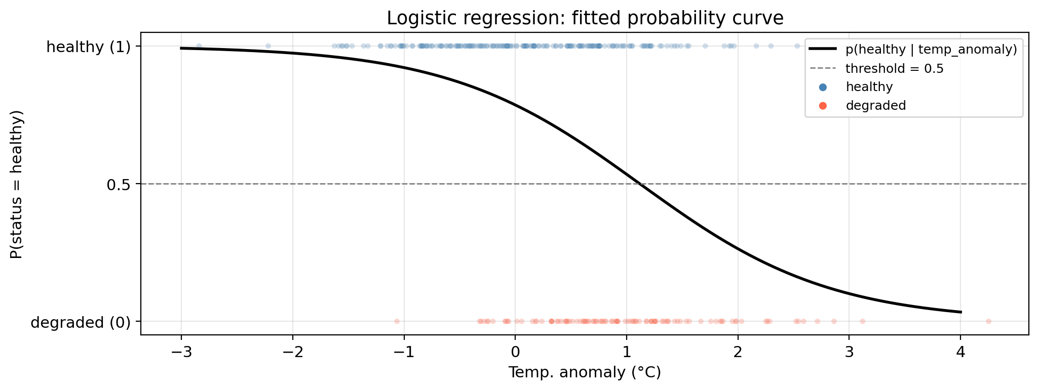
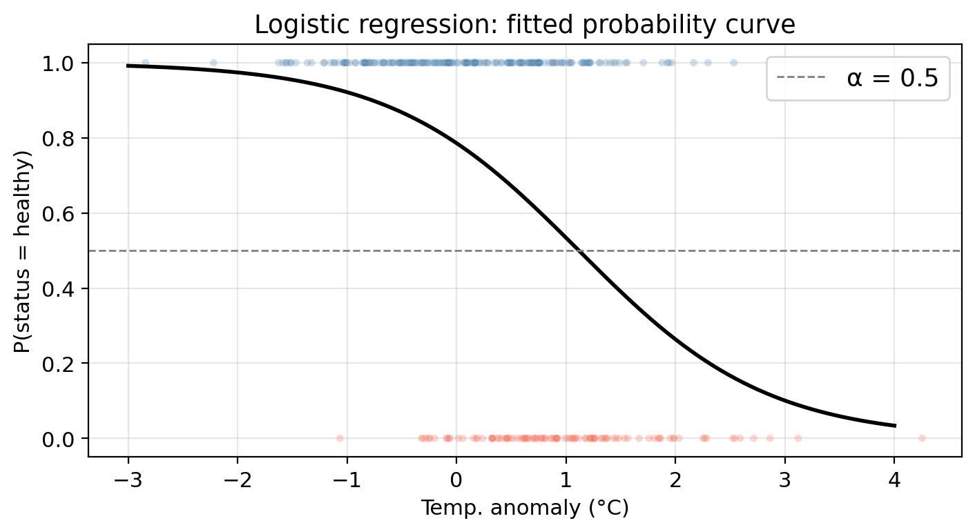
Fitted probability curve
- Points overlapping near the boundary reflects uncertainty in the data.
- Probability is higher in regions where healthy sites are dense
- As temperature anomaly increases, the probability of a healthy site decreases.
- Notice the characteristic S-shape of the logistic function!
Check-in
Using the fitted logistic model,
what is the predicted status of a site with temp_anomaly = 0.5°C? Use the threshold \(\alpha = 0.5\).
Check-in
Using the fitted logistic model,
what is the predicted status of a site with temp_anomaly = 0.5°C? Use the threshold \(\alpha = 0.5\).
Using the probability function we obtain \(p(0.5) = 0.6722\). Since this is above the classification threshold of 0.5, the site is predicted as ‘healthy’.
Interpreting the coefficients
Log-odds
- Logistic regression allows us to do both prediction and inference.
- Once we have fitted our model and estimated the coefficients \(\hat{\beta}_i\), we can interpret them to understand relations between predictor variables and response.
Starting from the logistic function
\[p(X) = \frac{e^{\beta_0 + \beta_1 X}}{1 + e^{\beta_0 + \beta_1 X}},\]
rearrange it to get the odds:
\[\frac{p(X)}{1 - p(X)} = e^{\beta_0 + \beta_1 X}.\]
Take the natural logarithm to get the log-odds:
\[\log\left(\frac{p(X)}{1 - p(X)}\right) = \beta_0 + \beta_1 X.\]
Log-odds
The log-odds are defined by
\[\log\left(\frac{p(X)}{1 - p(X)}\right) = \beta_0 + \beta_1 X.\]
Notice the log-odds is linear in \(X\).
In addition, \(p(X)\) changes in the same direction as the log-odds.
This helps us understand the relationship between \(X\) and \(p(X)\):
- If \(\hat\beta_1 > 0\), then
increasing \(X\) \(\Rightarrow\) log-odds increase \(\Rightarrow\) probability of belonging to positive class \(p(X)\) increases
- If \(\hat\beta_1 < 0\), then
increasing \(X\) \(\Rightarrow\) log-odds decrease \(\Rightarrow\) probability of belonging to positive class \(p(X)\) decreases
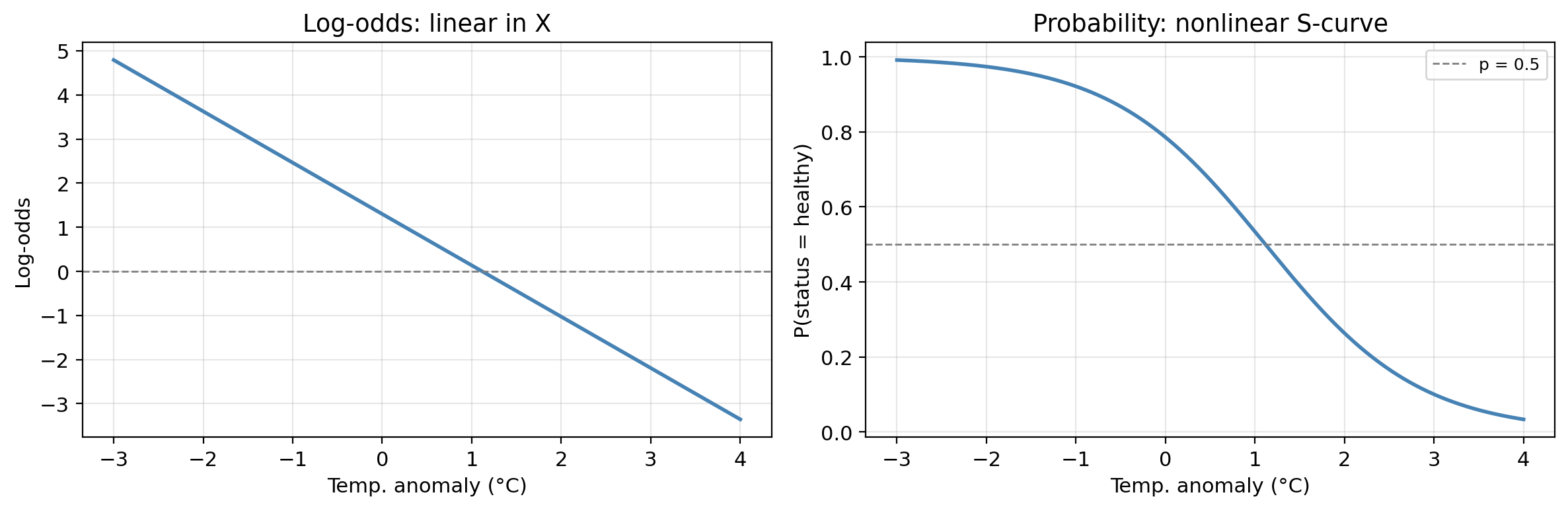
Log-odds and probability
The log-odds scale is linear; the probability scale is the familiar S-curve.
Both representations contain the same information.
Check-in
The fitted model has \(\hat{\beta}_0 =\) 1.300 and \(\hat{\beta}_1 =\) -1.164.
What does the sign of \(\hat{\beta}_1\) tell us about the relationship between temperature anomaly and kelp forest health?
A negative \(\hat\beta_1\) means that as temperature anomaly increases (warmer ocean conditions), the log-odds of a healthy site decrease, which implies the probability of healthy status decreases.
So warmer-than-average temperatures are associated with degraded kelp forests.
Is there evidence for a relationship between X and Y?
If \(\beta_1 = 0\), then:
\[p(X) = \frac{e^{\beta_0}}{1 + e^{\beta_0}} = \text{constant}\]
meaning the probability of the positive class does not depend on \(X\) at all.
Our hypotheses thus are:
- Null hypothesis \(H_0\): there is no relationship between \(X\) and \(p(X)\), i.e., \(\beta_1 = 0\).
- Alternative hypothesis \(H_a\): there is some relationship between \(X\) and \(p(X)\), i.e., \(\beta_1 \neq 0\).
We test this using the Z-statistic (analogue of the t-statistic in linear regression):
\[Z = \frac{\hat{\beta}_1}{\text{SE}(\hat{\beta}_1)}.\]
A large \(|Z|\) provides evidence against \(H_0\). The p-value quantifies how likely we would observe a Z-statistic this extreme if \(H_0\) were true.
Check-in
The table below shows the results for the logistic regression of status on temp_anomaly. What does the \(p\)-value for temp_anomaly tell us?
 Coefficient  Estimate  Std. Error  Z-statistic p-value
   Intercept    1.3000      0.1748        7.437  0.0000
temp_anomaly   -1.1639      0.1739       -6.693  0.0000
Very small \(p\)-value for temp_anomaly: strong evidence against \(H_0\): temperature anomaly is significantly associated with kelp forest status.
We reject \(H_0: \beta_1 = 0\): there is a real relationship between temperature anomaly and the probability of a site being healthy.
Multiple logistic regression
Multiple logistic regression
The logistic model extends naturally to multiple predictors \(X_1, X_2, \ldots, X_p\):
\[p(X) = \frac{e^{\beta_0 + \beta_1 X_1 + \cdots + \beta_p X_p}}{1 + e^{\beta_0 + \beta_1 X_1 + \cdots + \beta_p X_p}}.\]
The log-odds remain linear in all predictors:
\[\log\left(\frac{p(X)}{1 - p(X)}\right) = \beta_0 + \beta_1 X_1 + \cdots + \beta_p X_p.\]
Each coefficient \(\hat\beta_j\) represents the change in log-odds for a one-unit increase in \(X_j\), holding all other predictors constant:
- \(\hat\beta_j > 0\): increasing \(X_j\) \(\Rightarrow\) higher log-odds \(\Rightarrow\) higher \(p(X)\) (holding other predictors fixed)
- \(\hat\beta_j < 0\): increasing \(X_j\) \(\Rightarrow\) lower log-odds \(\Rightarrow\) lower \(p(X)\) (holding other predictors fixed)
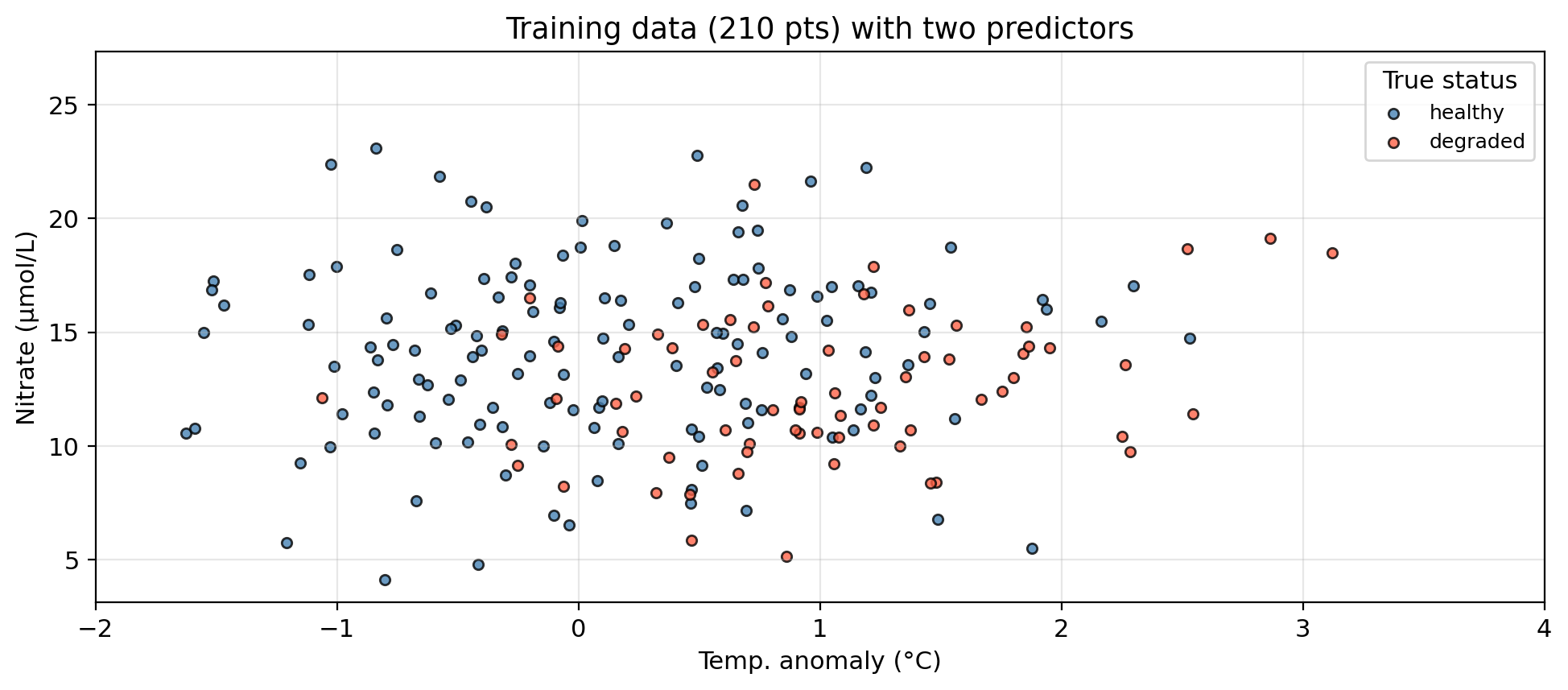
Multiple logistic regression: example data
In our example:
- Predictors:
temp_anomaly, nitrate
- Response:
status: healthy (class 1/positive) or degraded (class 0/negative)
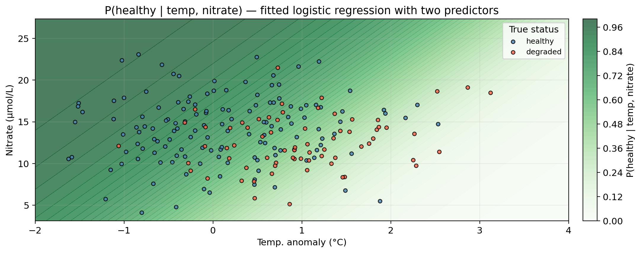
Using logistic regression we can model
\[P(\text{status} = \text{healthy} \mid \text{temp_anomaly}, \text{nitrate}) = p(\text{temp_anomaly}, \text{nitrate}),\]
the probability of a site having a healthy status given a certain temperature anomaly and nitrate concentration.
Then, we select a threshold to classify a site as healthy or degraded. E.g., using \(\alpha=0.5\):
- If \(p(\text{temp_anomaly}, \text{nitrate}) \geq 0.5\), then predict the site is healthy.
- If \(p(\text{temp_anomaly}, \text{nitrate}) < 0.5\), then predict the site is degraded.
Logistic regression with two predictors
Logistic regression with two predictors
Darker green = higher predicted probability of healthy status.
Logistic regression with two predictors
Darker green = higher predicted probability of healthy status.
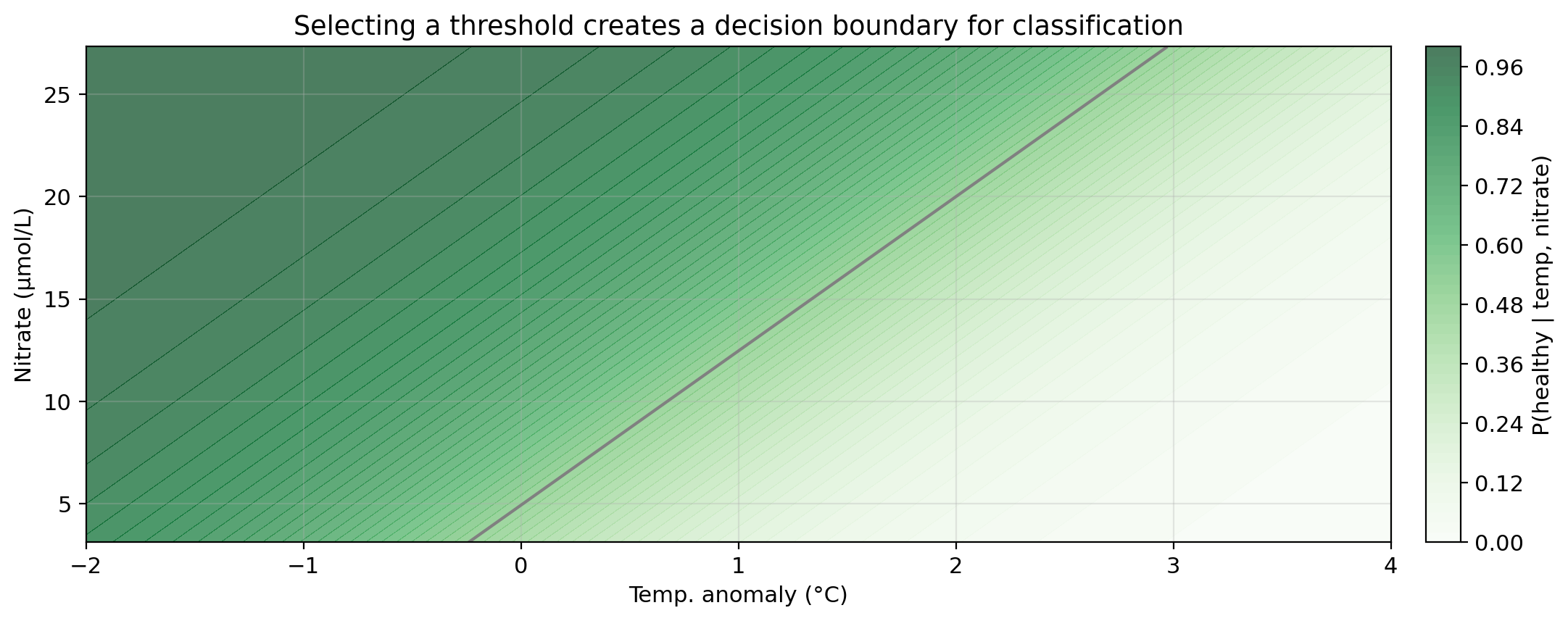
Logistic regression with two predictors
Darker green = higher predicted probability of healthy status.
Gray line = decision boundary using the threshold \(\alpha = 0.5\).
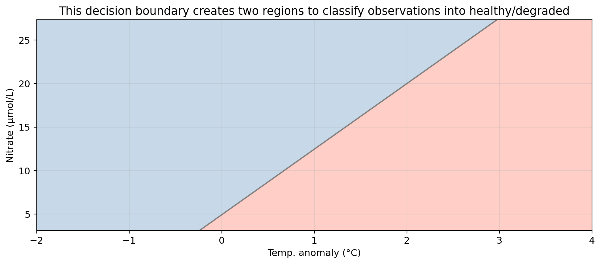
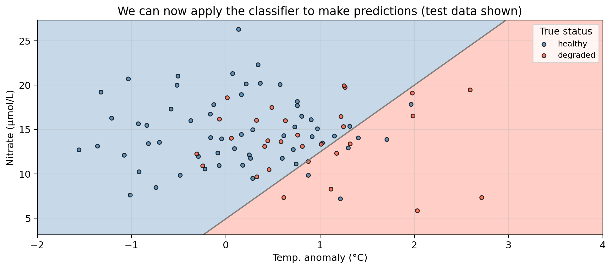
Logistic regression with two predictors
Blue region = predicted healthy, red region = predicted degraded.
Gray line = decision boundary using the threshold \(\alpha = 0.5\).
Logistic regression with two predictors
Blue region = predicted healthy, red region = predicted degraded.
Gray line = decision boundary using the threshold \(\alpha = 0.5\).
Points in the “wrong” region are misclassified.
Adjusting the classification threshold
Adjusting the classification threshold
The default threshold \(\alpha = 0.5\) is just a convention. We can choose any value between 0 and 1.
Suppose the threshold is raised to \(\alpha = 0.9\). What type of error (FP or FN) would you expect more of, and what does this mean for precision and recall? Now repeat for \(\alpha = 0.2\).
\(\alpha = 0.9\): Only sites with very high predicted probability are classified as healthy. Many truly healthy sites fall below this bar and are classified as degraded → many false negatives. Precision increases (when we do predict healthy, we’re usually right), but recall falls.
\(\alpha = 0.2\): Almost every site is classified as healthy. Most truly healthy sites are caught → very few false negatives → high recall. But many degraded sites are also classified as healthy → many false positives → precision
Adjusting the classification threshold
Changing the threshold has a tradeoff between recall and precision:
Raising the classification threshold means fewer observations get predicted as positive: precision increases, recall decreases (more false negatives).
Lowering the classification threshold means more observations get predicted as positive: recall increases, precision decreases (more false positives).
There is no single correct answer and the selection must be guided by:
- Domain knowledge: what is the consequence of each error type?
- The precision–recall tradeoff: understanding what you gain and lose at each threshold.
- Cross-validation: evaluating threshold performance on held-out data rather than the test set (more on this on next lesson).
Check-in
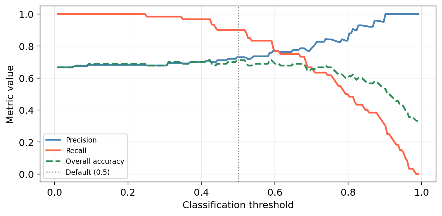
The graph below shows the precision, recall, and overall accuracy for our multiple logistic regression kelp forest status classifier at different classification threshold levels.
What would we miss by evaluating performance using only overall accuracy?
Check-in
The graph below shows the precision, recall, and overall accuracy for our multiple logistic regression kelp forest status classifier at different classification threshold levels.
What would we miss by evaluating performance using only overall accuracy?
Overall accuracy hides the precision–recall tradeoff.
A threshold that maximizes accuracy may still have poor recall (missing many healthy sites) or poor precision (flagging many degraded sites).
The green dashed line barely changes across a wide range of thresholds, but precision and recall shift a lot!
ROC curves
The ROC curve plots two metrics against each other across all possible thresholds.
It uses the following metrics:
True Positive Rate (TPR) = Recall
\[TPR = \frac{TP}{TP + FN}\]
Of all truly healthy sites, what fraction did we correctly identify?
False Positive Rate (FPR)
\[FPR = \frac{FP}{FP + TN}\]
Of all truly degraded sites, what fraction did we incorrectly flag as healthy?
We obtain the ROC curve by calculating the TPR and the FPR at every value classification threshold and then plotting TPR with respect to FPR.
Check-in
We obtain the ROC curve by calculating the TPR and the FPR at every value classification threshold and then plotting TPR with respect to FPR.
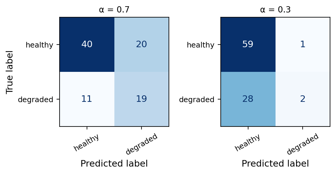
Use the confusion matrices to fill in the table. Then sketch the ROC curve through those points.
Check-in
  α   TPR   FPR
1.0 0.000 0.000
0.7 0.667 0.367
0.3 0.983 0.933
0.0 1.000 1.000
- \(\alpha = 1.0\): all predicted negative → TPR = FPR = 0 → point (0, 0)
- \(\alpha = 0.0\): all predicted positive → TPR = FPR = 1 → point (1, 1)
The curve always goes from (0, 0) to (1, 1).
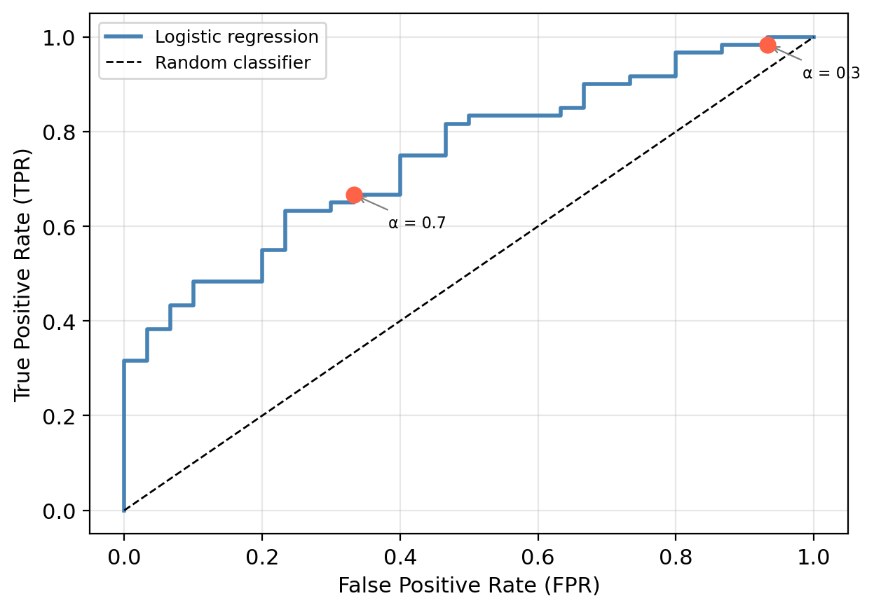
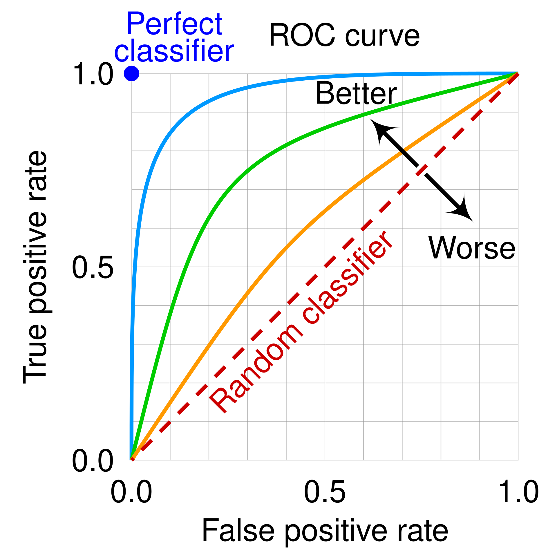
Reading the ROC curve
- Perfect classifier: passes through (0, 1). Zero false positives with perfect recall
- Random classifier: the diagonal. No better than a coin flip
- Closer to upper-left: better discriminating ability. This is what we aim for
Lowering the threshold raises both TPR and FPR.
We gain recall at the cost of more false positives.
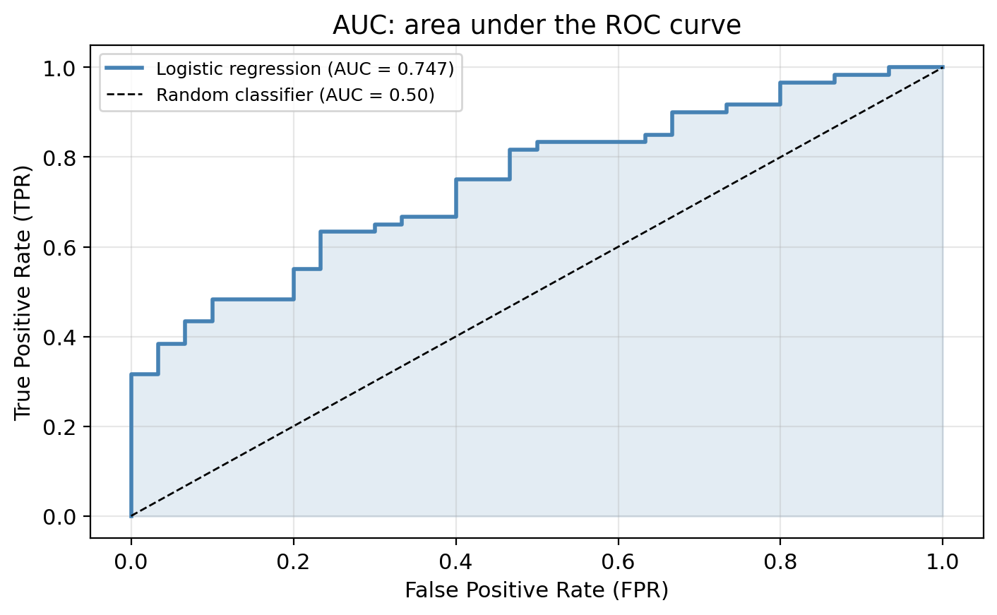
Area under the curve (AUC)
The AUC summarizes the entire ROC curve in a single number. Mostly used to compare models.
| 1.0 |
Perfect classifier |
| > 0.8 |
Good discriminating ability (in most applications) |
| > 0.5 |
Some discriminating ability |
| 0.5 |
Random classifier (no better than a coin flip) |
Check-in
A colleague proposes a model with AUC = 0.52. Would you use it over the logistic regression? Why or why not?
Check-in
A colleague proposes a model with AUC = 0.52. Would you use it over the logistic regression? Why or why not?
A model with AUC = 0.52 is barely better than random and almost certainly not useful in practice. The logistic regression would be preferred.