EDS 232
Lesson 8
Linear model selection and regularization
In this lesson
- The problem of variable selection in multiple linear regression
- Shrinkage methods
- Ridge regression and the lasso
- How to use cross-validation to select the tuning parameter \(\lambda\) for both methods
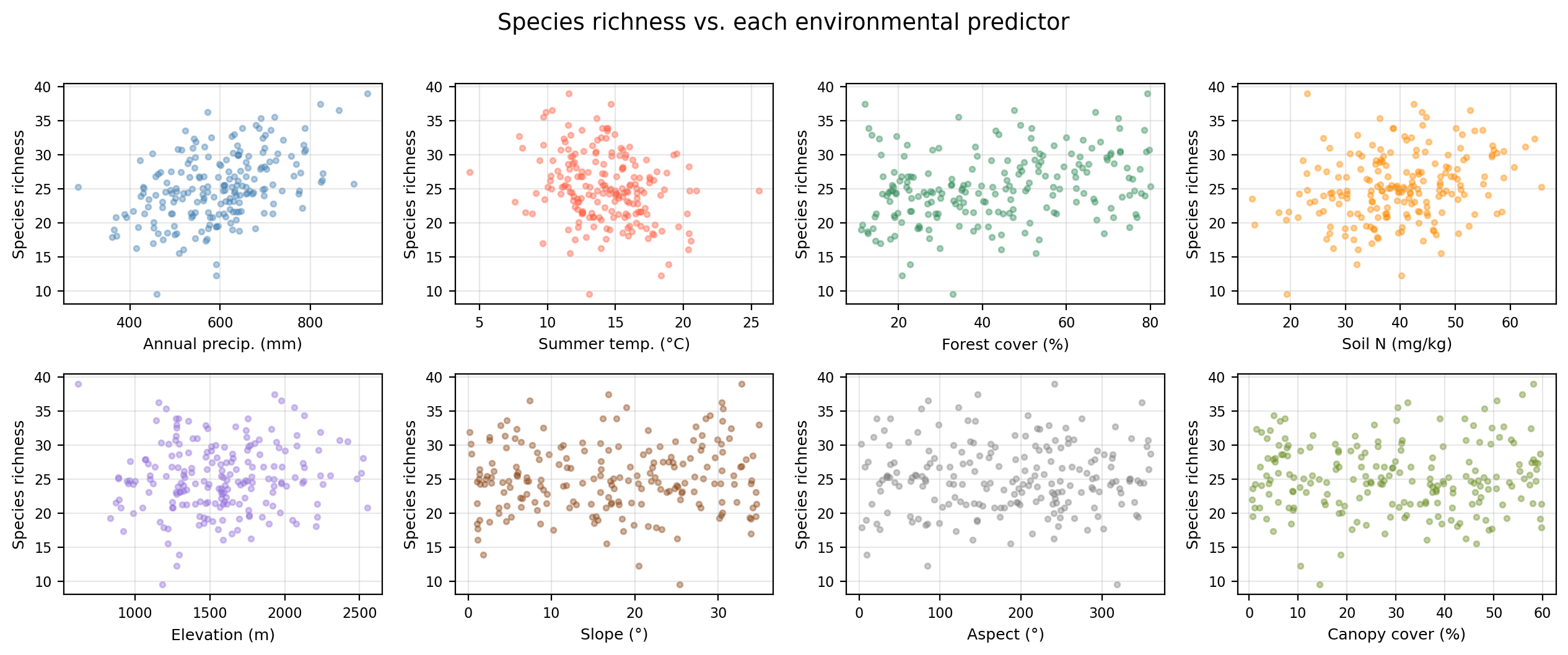
Our example dataset
200 mountain meadow survey plots.
We want a simple, efficient model good at predicting the response, with the feweset possible variables.
Data overview
Synthetic data generated for educational purposes only
The MLR set up
In the MLR model we assume: \(Y = \beta_0 + \beta_1 X_1 + \beta_2 X_2 + \cdots + \beta_p X_p + \epsilon.\)
Our goal is to estimate the coefficients and obtain a model
\[\hat{Y} = \hat{\beta}_0 + \hat{\beta}_1 X_1 + \hat{\beta}_2 X_2 + \cdots + \hat{\beta}_p X_p.\]
Our training set is \(\{(x_1, y_1), \ldots, (x_n, y_n)\}\) with \(n\) observations.
For each of the observations \((x_i, y_i)\) we have that:
- \(x_i = (x_{i1}, x_{i2}, \ldots, x_{ip})\) is a vector of \(p\) predictor values, and
- \(y_i\) is the response associated to \(x_i\).
We estimate the coefficients/fit the model by finding the \(\hat{\beta}_i\) that minimize the residual sum of squares:
\[
RSS = \sum_{i=1}^{n} (y_i - \hat{y}_i)^2.
\]
Variable selection
After fitting a multiple linear regression we check:
- The \(F\)-statistic and its \(p\)-value: is there evidence that any predictor matters?
- Individual \(p\)-values: which predictors are associated with the response, assuming all others are also in the model?
If some predictors are important, the key question is: which predictors should we include?
- Including unnecessary predictors increases variance without improving fit
- Leaving out important predictors biases our estimates
What would be a straightforward way to find which subset of the predictors \(X_1, \ldots, X_p\) will give us the best model?
With \(p\) predictors there are \(2^p\) possible ways of choosing which predictors to use:
- \(p = 3\): 8 models — feasible to compare exhaustively
- \(p = 8\): 256 models
- \(p = 30\): over 1 billion models — completely infeasible
What is regularization?
Variable selection searches over subsets: keeping some predictors, discarding others.
Shrinkage methods: keep all \(p\) predictors but alter the fitting method itself so that it naturally shrinks less important coefficients towards zero.
Check-in
In the linear model
\[Y = \hat{\beta}_0 + \hat{\beta}_1 X_1 + \cdots + \hat{\beta}_p X_p,\]
how would you “remove” a predictor \(X_i\) by changing its coefficient estimate?
Set \(\hat{\beta}_i = 0\). Then the contribution \(\hat{\beta}_i X_i = 0 \cdot X_i = 0\). So \(X_i\) has no effect on predictions, equivalent to removing it from the model.
The penalized objective
Remember the usual fit of the MLR model is done by minimizing
\[\text{minimize} \quad ( RSS + \text{penalty})\]
Instead of minimizing RSS alone, regularization fits MLR by minimizing:
\[\text{minimize} \quad ( RSS + \text{penalty})\]
The penalty term:
- Is small when \(\beta_1, \ldots, \beta_p\) are close to zero
- Constrains coefficient size: they can only grow if accompanied by a sufficient reduction in RSS
- Discourages model complexity
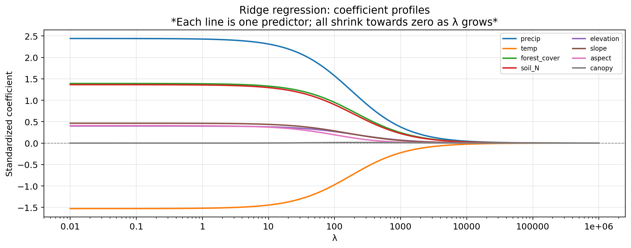
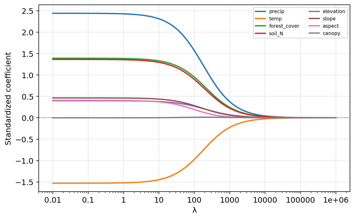
Ridge coefficient profiles
Check-in
Which predictors appear most important (retain the largest coefficients as \(\lambda\) increases, i.e. are most resistant to shrinkage)?
You have fit ridge at a grid of \(\lambda\) values and obtained a different set of coefficient estimates for each. What method would you use to select a good \(\lambda\)?
Check-in
Which predictors appear most important (coefficient’s magnitude remains large as \(\lambda\) increases, i.e. are most resistant to shrinkage)?
You have fit ridge at a grid of \(\lambda\) values and obtained a different set of coefficient estimates for each. What method would you use to select a good \(\lambda\)?
precip, and temp retain the largest coefficients as \(\lambda\) increases, so they appear to be the most important predictors. aspect and canopy seem to be irrelevant as they stay near zero across the entire range.
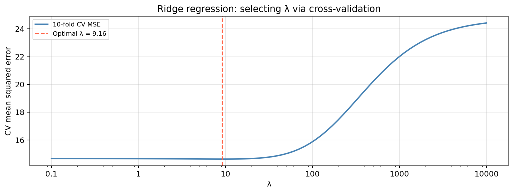
Use \(k\)-fold cross-validation!
Selecting the tuning parameter
Small \(\lambda\): close to OLS, may overfit. Large \(\lambda\): too constrained, underfits. The optimal \(\lambda\) balances these extremes.
Check-in
The lasso regression finds the estimates of the coefficients \(\hat{\beta}_i\) by minimizing::
\[RSS + \underbrace{\lambda \sum_{j=1}^{p} |\beta_j|}_{\text{ penalty}}.\]
If \(\lambda = 0\), how are the lasso coefficient estimates related to the least squares estimates?
What happens to all lasso coefficients when \(\lambda\) is very large?
When \(\lambda = 0\) there is no penalty, so minimizing \(RSS + 0 \cdot \sum |\beta_j|\) is the same as minimizing RSS alone. The lasso estimates equal the OLS estimates.
As \(\lambda \to \infty\) the penalty dominates and forces all coefficients to exactly zero. The model reduces to the null model (intercept only), predicting the mean response for every observation.
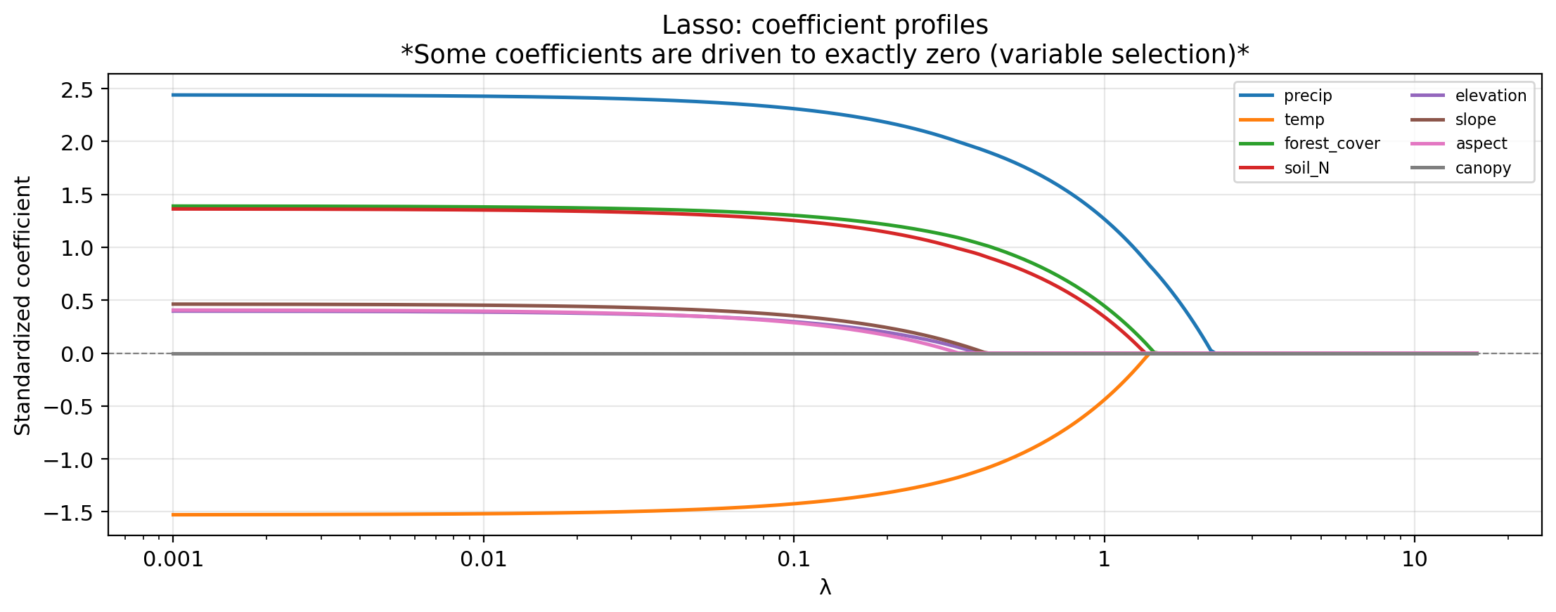
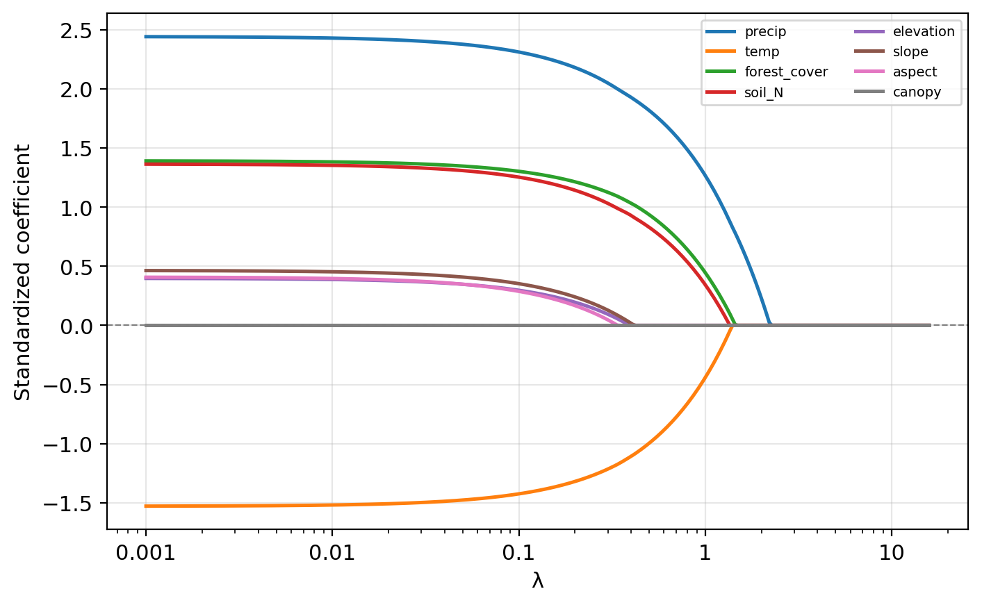
Lasso coefficient profiles
Check-in
Based on the lasso coefficient profile plot, which predictors are driven to exactly zero first as \(\lambda\) increases?
Check-in
Based on the lasso coefficient profile plot, which predictors are driven to exactly zero first as \(\lambda\) increases?
aspect and canopy are driven to exactly zero at the smallest \(\lambda\) values, followed by elevation and slope. Their coefficient lines flatten to zero and stay there.
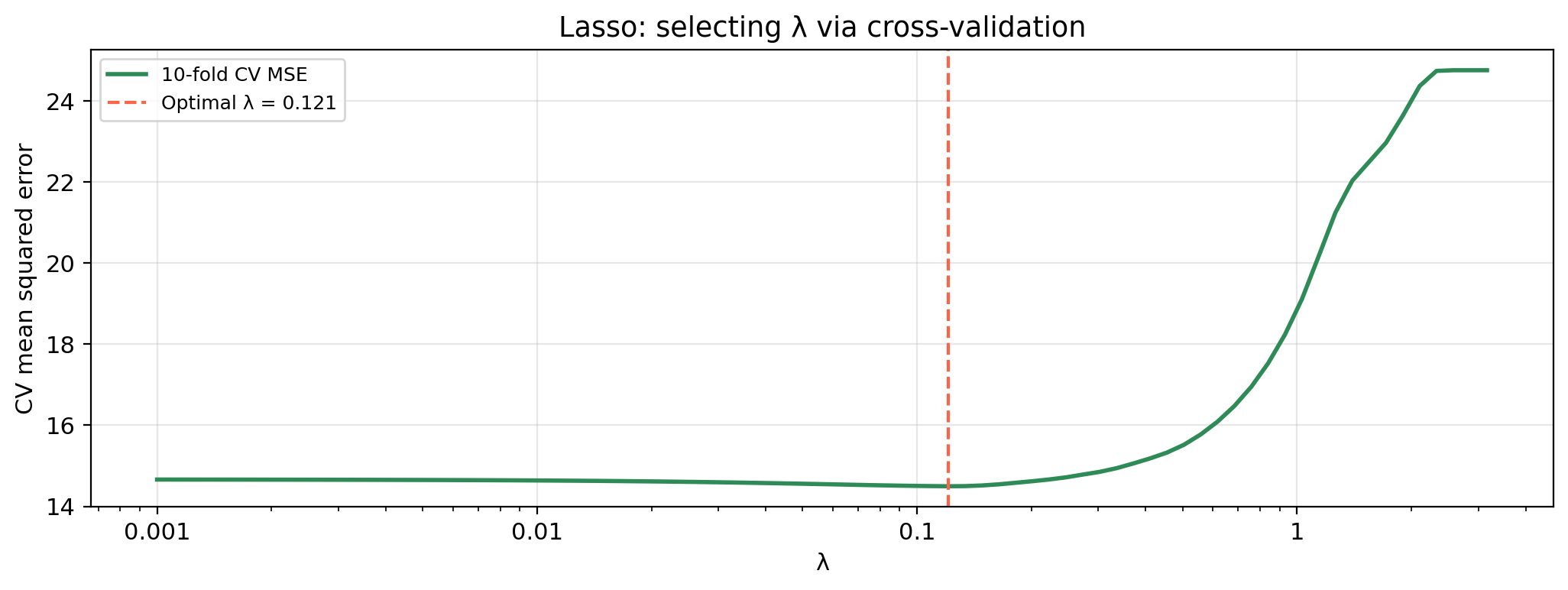
Selecting the tuning parameter
The lasso tuning parameter is selected by the same 10-fold CV procedure as ridge: fit at many \(\lambda\) values, compute CV-MSE at each, select the minimum.
Comparing lasso and ridge
When to use each
Neither method consistently outperforms the other:
- Prefer lasso when the response depends on a small number of strong predictors (sparse setting). The resulting model is sparser and easier to interpret.
- Prefer ridge when the response depends on many predictors, each contributing a roughly equal amount (dense setting). Lasso may incorrectly discard informative predictors in this case.
The number of truly relevant predictors is never known in advance for real data.
Cross-validation can be used to compare both approaches and select the one with lower CV-MSE.
Check-in
   Predictor  True β    OLS  Ridge (CV λ)  Lasso (CV λ)
      precip    2.50  2.442         2.323         2.283
        temp   -1.80 -1.529        -1.453        -1.402
forest_cover    1.50  1.391         1.335         1.284
      soil_N    1.00  1.364         1.301         1.230
   elevation    0.50  0.398         0.381         0.276
       slope    0.15  0.464         0.439         0.329
      aspect    0.00  0.408         0.375         0.263
      canopy    0.00 -0.001         0.002         0.000
How do ridge and lasso estimates compare to the true \(\beta\) for precip, temp, forest_cover, and soil_N?
What has lasso done to canopy? What has ridge done?
Both methods shrink estimates towards zero relative to OLS, but they recover the correct ranking and signs for the four important predictors.
Lasso sets canopy to exactly zero: correctly identifies it as irrelevant. Ridge retains both with small but non-zero coefficients.