EDS 232 - Machine Learning for Environmental Science

EDS 232

Lesson 9

Bagging and Random Forests

In this lesson

Ensemble methods
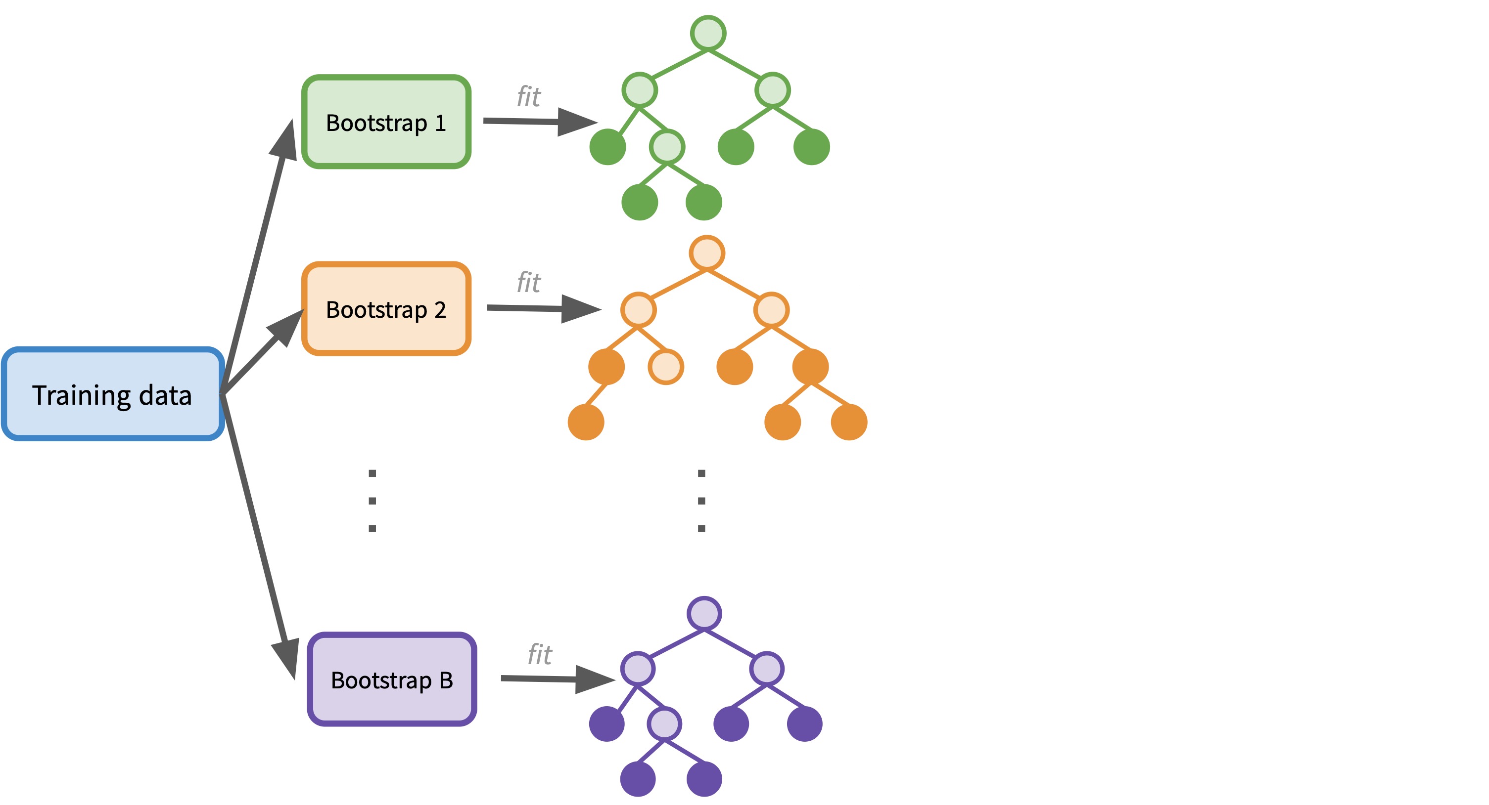
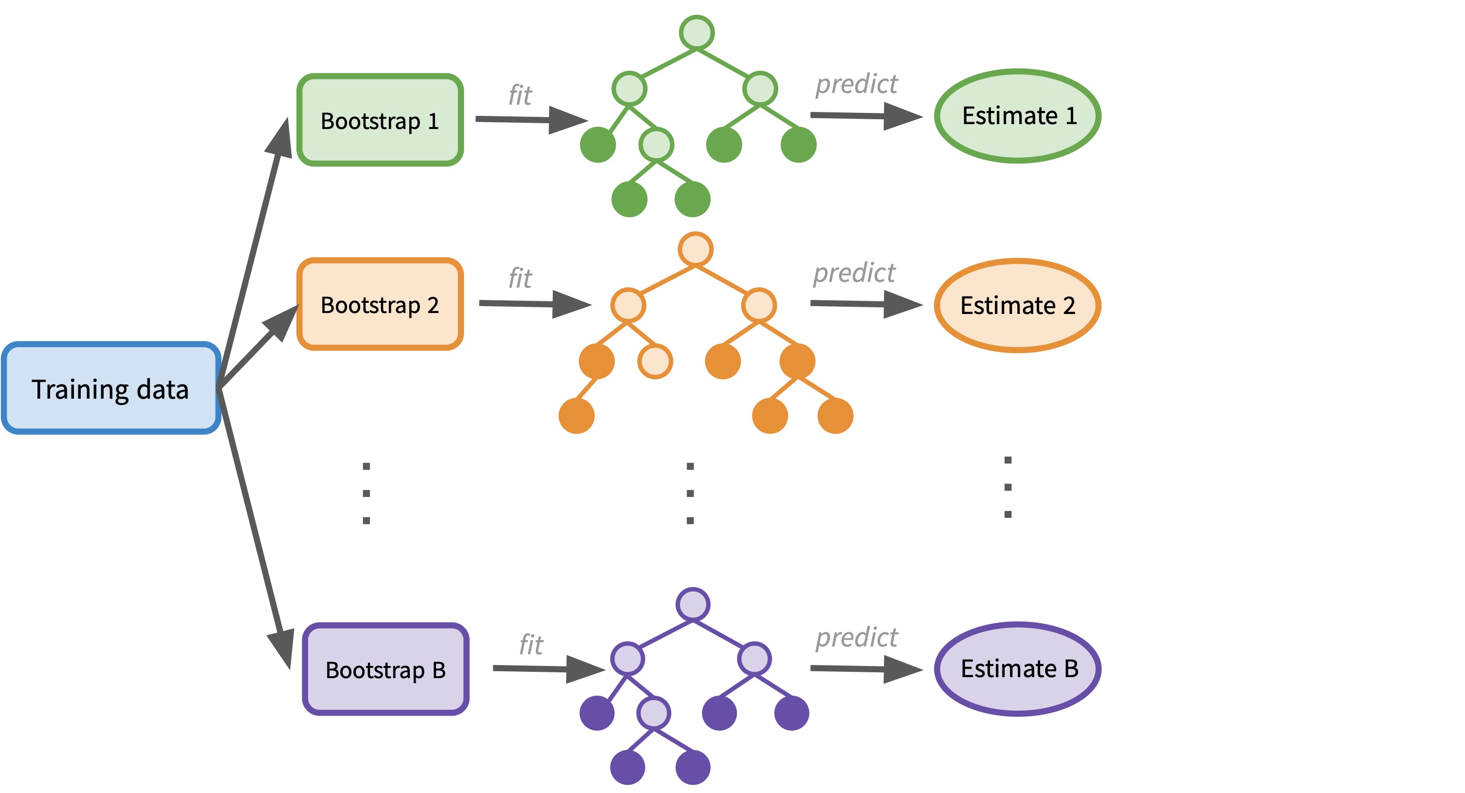
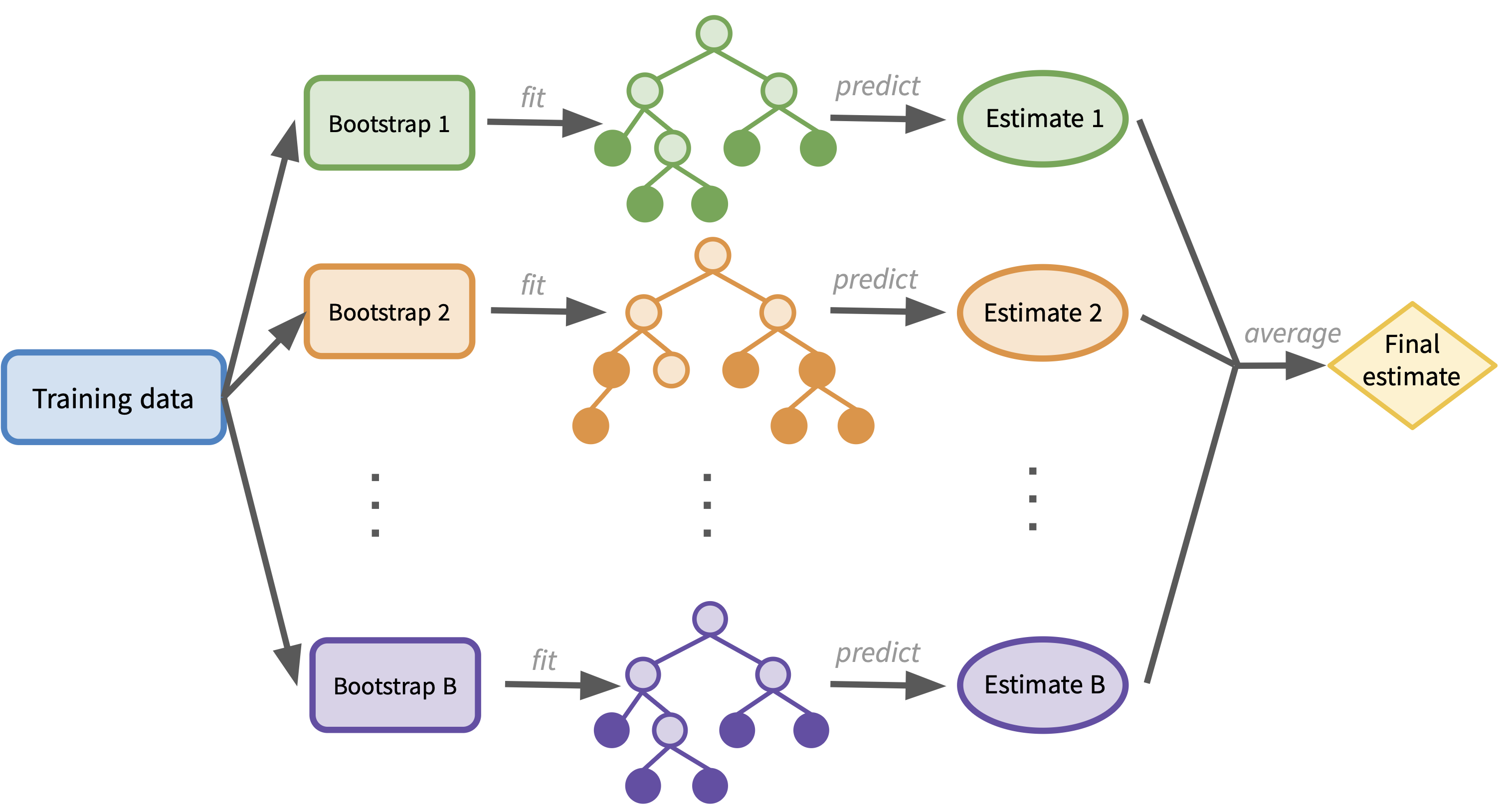
Bagging: fitting many trees on bootstrap samples and averaging predictions
Out-of-bag error estimation: an alternative to cross-validation
Random forests: decorrelating trees by using a random subset of predictors at each split

A guiding dataset

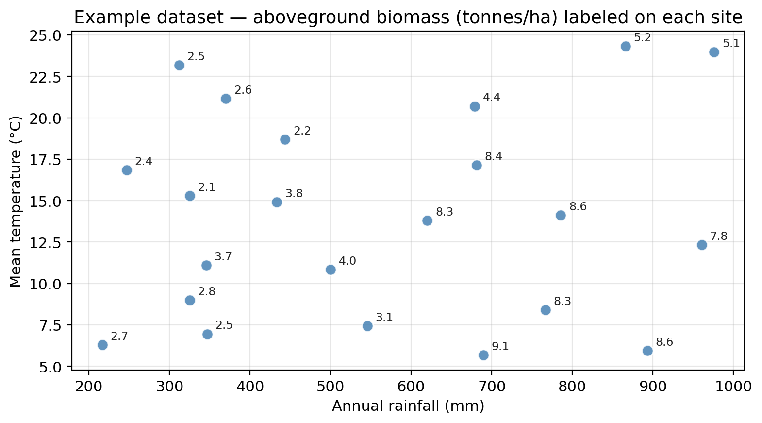
22 ecological survey sites, each characterized by:

rainfall — annual precipitation (mm)
temperature — mean summer temperature (°C)
biomass — aboveground plant biomass (tonnes/ha) (response)

The variance problem in decision trees

A single decision tree suffers from high variance: small changes in the training data can lead to very different trees and very different predictions. Deep trees are prone to overfitting.

One general strategy for reducing variance:

Take many training sets from the same population
Fit a separate model on each training set
Average the resulting predictions

Core idea: The more uncorrelated the individual predictions are, the more variance reduction we get from averaging.

The challenge: in practice we only have a single training set. Bootstrapping is a way around this.

Bootsrapping & bagging

Bootsrap

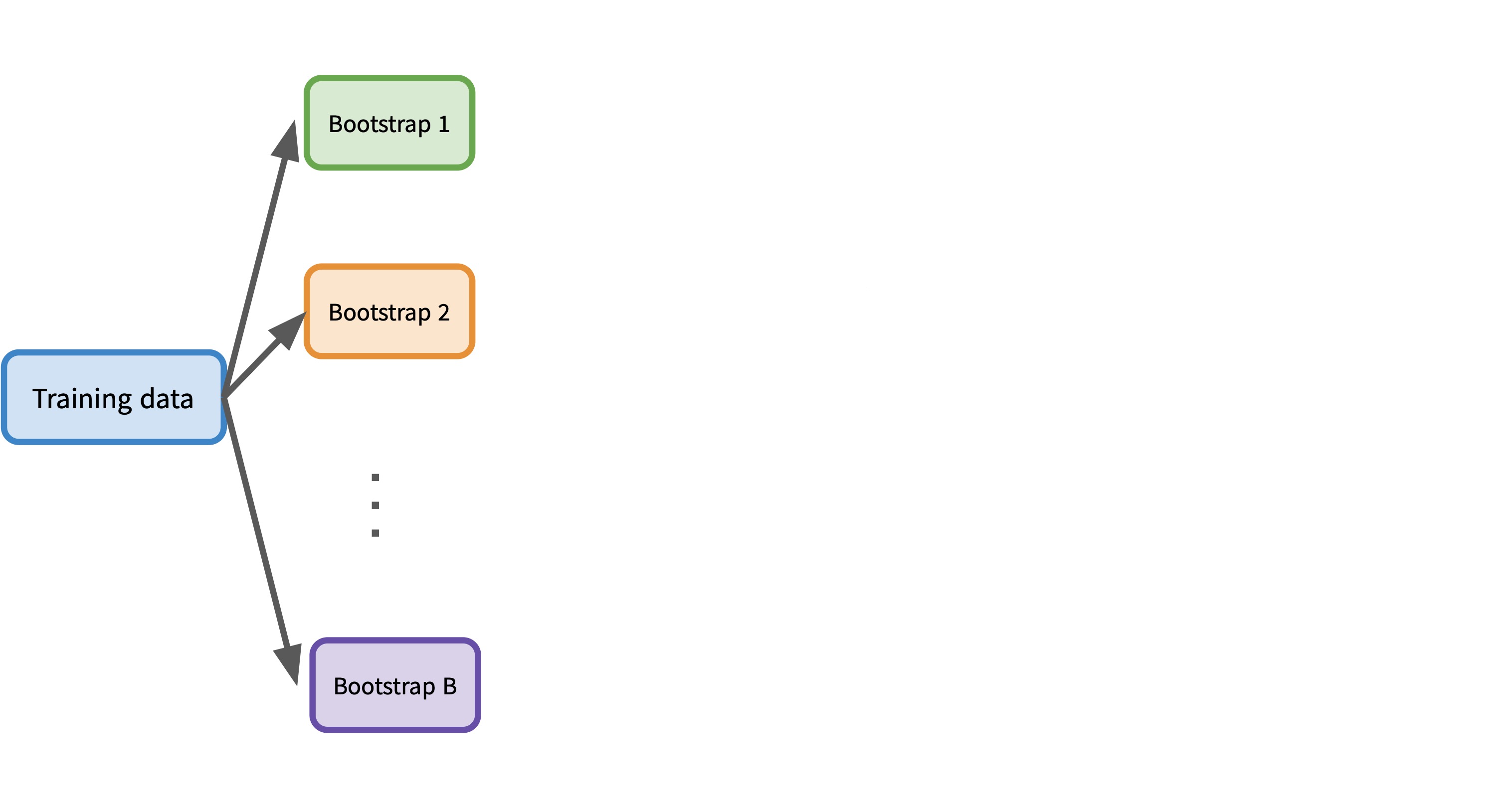
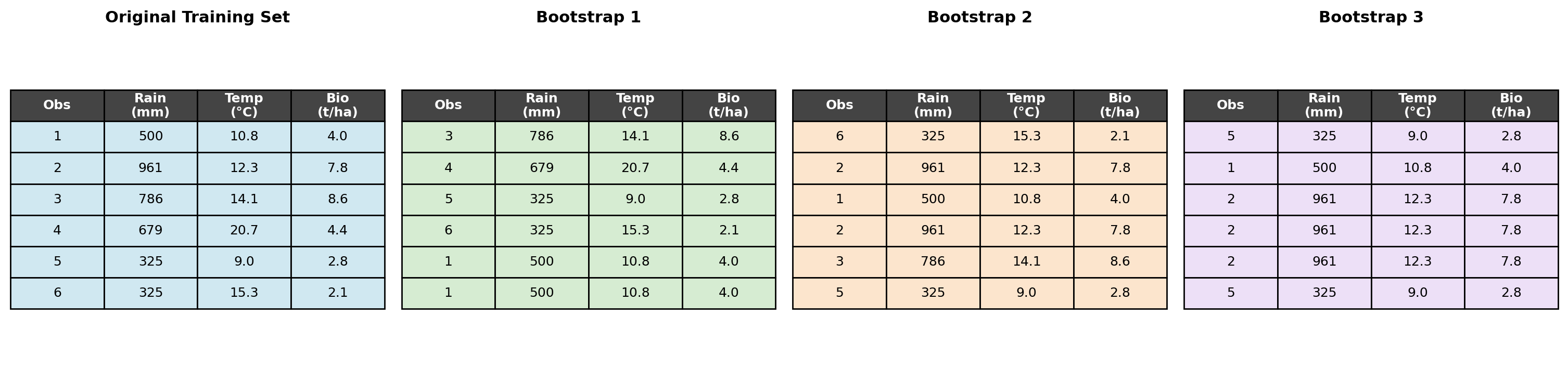
Bootstrapping: generate a new training set by sampling with replacement from the original training set

Each bootstrapped sample is the same size as the original
Some observations appear more than once
Some observations are left out entirely

Bagging — Bootstrap AGGregatING

Bagging is a method to generate an ensemble model by:

Generating many training sets from the single one we have by bootstrapping
Fitting a model on each bootstrapped sample
Then aggregate predictions to get a final prediction from the ensemble

Bagging for regression

Generate \(B\) bootstrapped training sets
Fit a decision tree on each bootstrapped training set
Obtain \(B\) estimates \(\hat{f}^{*1}(x), \ldots, \hat{f}^{*B}(x)\), one for each tree
Average the predictions:

\[\hat{f}_{\text{bag}}(x) = \frac{1}{B} \sum_{b=1}^{B} \hat{f}^{*b}(x)\]

Check-in

How would you modify the bagging workflow for a classification problem? What changes? Create the corresponding diagram.

Bagging for classification

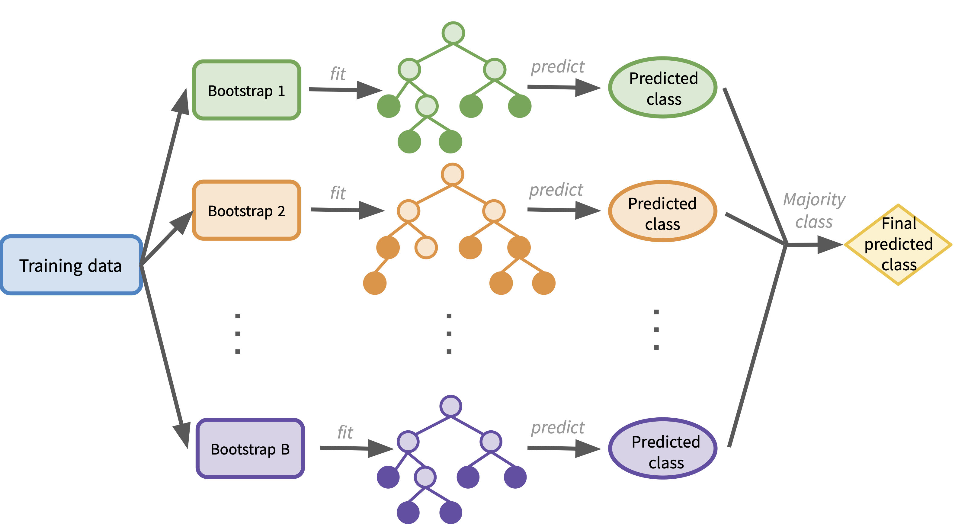
In the case of classification, the workflow is the same as the regression case, but the final aggregation step changes:

Instead of averaging numerical predictions, take a majority vote across all \(B\) trees
The final prediction is the most commonly occurring class:

Out-of-bag error estimation

Out-of-bag observations

When fitting each bootstrapped tree, some of the training observations are left out of that bootstrap sample. These are called the out-of-bag (OOB) observations for that tree.

Suppose your model has three trees fit on Bootstrap samples 1, 2, and 3 shown here. For which trees would observation 4 be an OOB observation?

Out-of-bag observations

When fitting each bootstrapped tree, some of the training observations are left out of that bootstrap sample. These are called the out-of-bag (OOB) observations for that tree.

Suppose your model has three trees fit on Bootstrap samples 1, 2, and 3 shown here. For which trees would observation 4 be an OOB observation?

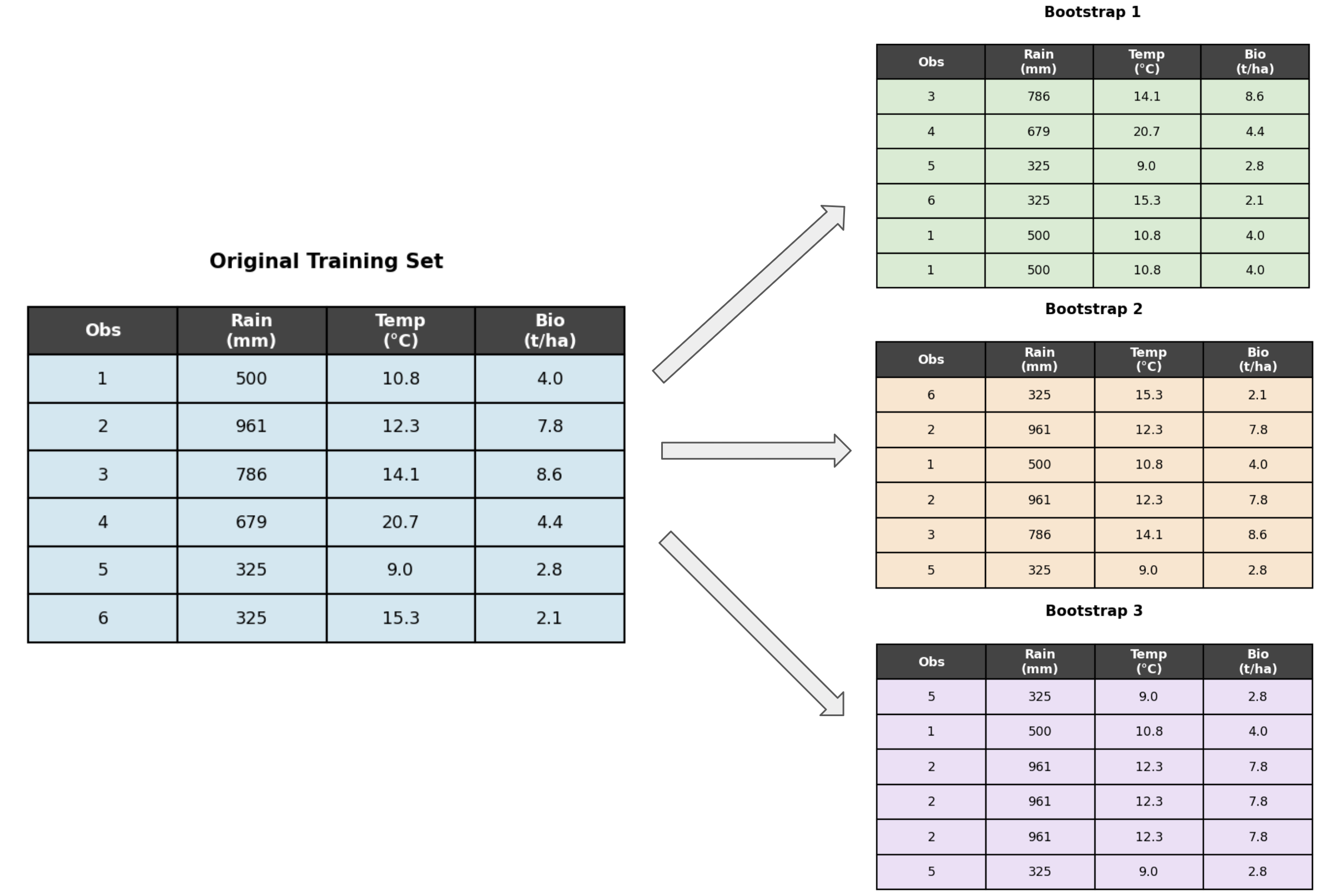
Observation 4 does not appear in Bootstrap samples 2 and 3, so it is an OOB observation for those two trees.

Out-of-bag error

OOB observations give us a way to estimate test error without cross-validation:

For each observation \((x_i, y_i)\), identify all trees for which it was OOB
Use only those trees to predict \(x_i\) (average for regression, majority vote for classification)
Repeat for all \(n\) training observations: get one OOB prediction per observation
Compute MSE (regression) or classification error from these OOB predictions

The OOB error is valid because each observation is predicted only by trees that were not trained on it.

We can use this error estimate to examne model parameters such as the number of trees.

Choosing the number of trees B

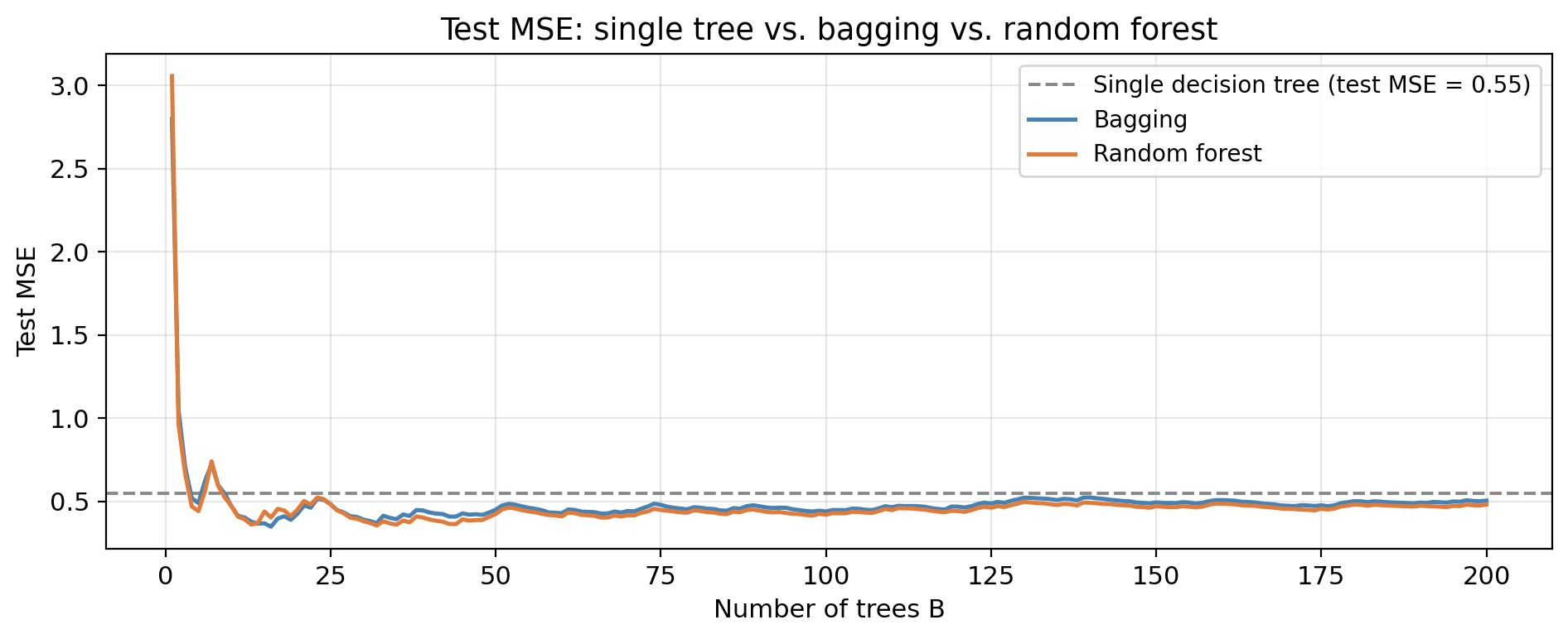
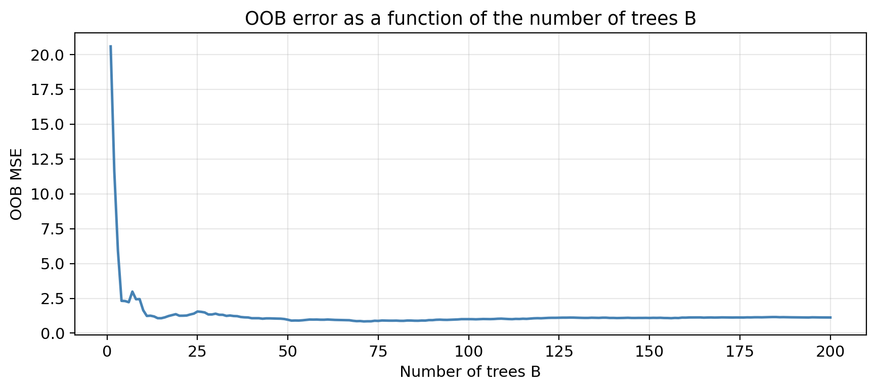
Unlike tree depth, \(B\) is not a regularization parameter. A very large \(B\) does not cause overfitting.

We pick a \(B\) large enough that the OOB error stabilizes. 100 to 500 are common defaults.

Variable importance

With \(B\) trees we lose the direct interpretability of a single tree diagram. But we can still extract a useful summary of which predictors matter most.

For each predictor, record the total reduction in RSS (regression) or Gini impurity (classification) achieved by splits on that predictor, averaged over all \(B\) trees.

Predictors with larger average reductions are more important to the model’s predictions.

Check-in

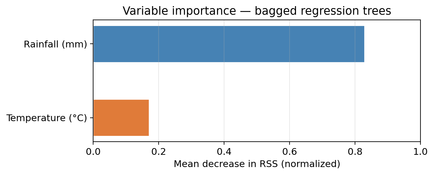
The plot shows variable importance for a model of bagged regression trees (B=200) on our example data.

Which predictor is most important for predicting biomass?
When creating the trees for the ensemble, which predictor would you expect to be used in the first split for most of them?

Check-in

The plot shows variable importance for a model of bagged regression trees (B=200) on our example data.

Which predictor is most important for predicting biomass?
When creating the trees for the ensemble, which predictor would you expect to be used in the first split for most of them?
Rainfall: it has the largest average RSS reduction across all trees.
Rainfall: consistent with the decision tree lesson, where the root node always split on rainfall first.

Random forests

Random forests: decorrelating the trees

Problem with bagging:

if one predictor is very strongly associated with the response, nearly every tree will use it as the top split
the \(B\) trees look similar
they are correlated
averaging correlated predictions does not reduce variance much.

Random forests fix this by introducing randomness at each split:

For every tree, at each split, randomly select a subset of \(m < p\) predictors as candidates
A fresh random subset is drawn at every split
Typical defaults: \(m = \sqrt{p}\) (classification), \(m = p/3\) (regression)

No single strong predictor can dominate every tree → trees are more diverse → averaging produces a larger reduction in variance.

Check-in

Suppose you are building one tree in a random forest with predictors {rainfall, temperature, elevation, soil moisture} (\(p = 4\), \(m = 2\)).

At the root node the algorithm randomly selects {rainfall, elevation} and splits on rainfall.

At the next node, which predictors are available to split on?

A new random sample of 2 predictors is drawn independently: it could be any pair, including ones used before. The previous split does not restrict future splits.

Random forest vs. bagging vs. single tree

Check-in

If \(m = p\) (we use all predictors at every split), how does a random forest relate to bagging?
When would you expect a random forest to outperform bagging the most?

When \(m = p\), random forests reduce to bagging exactly. There is no restriction on which predictors can be considered, so every tree is built the same way as a bagged tree.
When there are one or a few dominant predictors: bagged trees become too similar to each other, while random forests force diversity by sometimes excluding the dominant predictor from consideration.