EDS 232
Lesson 9
Decision Trees
In this lesson
- Decision trees: flexible, interpretable prediction models that partition the predictor space into rectangular regions
- Regression trees: decision trees for predicting a numerical response variable
- Classification trees: decision trees for predicting a categorical class label
- Dealing with overfitting: approaches for controlling model complexity
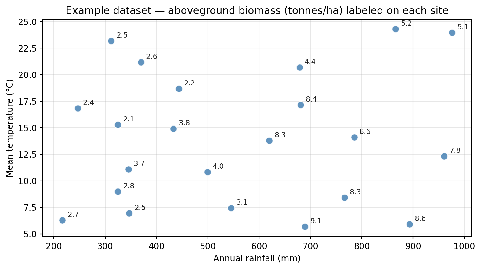
A guiding dataset
22 ecological survey sites, each characterized by:
rainfall — annual precipitation (mm)temperature — mean summer temperature (°C)biomass — aboveground plant biomass (tonnes/ha) (response)
What is a regression tree?
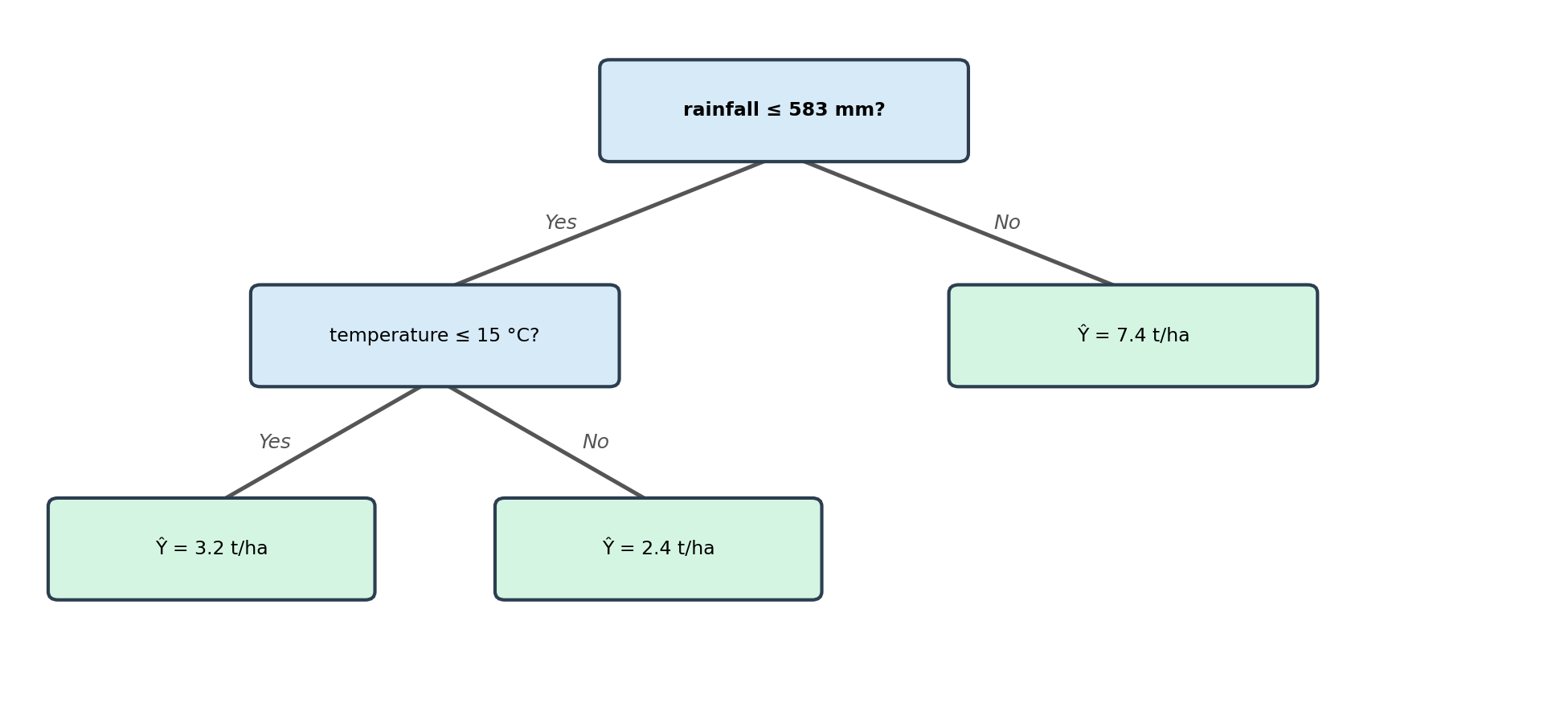
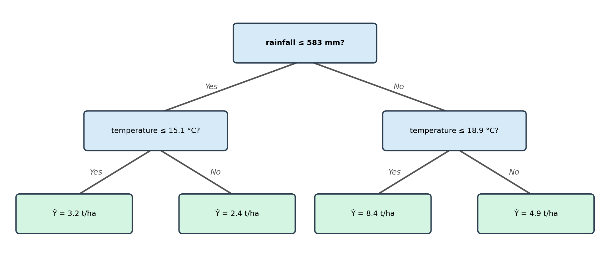
Regression tree structure
A regression tree predicts a numerical response by partitioning the predictor space into rectangular regions and assigning a predicted value to each region.
Tree terminology
- Root node: first split, applied to the entire dataset
- Internal node: a non-leaf node that applies an additional split to a subset
- Leaf node: a terminal node — no further splits
- Branch: the path an observation takes at each split
- Depth: number of nodes along the longest root-to-leaf path
The predicted value at a leaf is the mean response of all training observations that reach that leaf.
Making predictions
To predict for a new observation: start at the root and follow the branches based on the split conditions until reaching a leaf. The value at the leaf is the prediction.
For example, a new site with rainfall = 430 mm and temperature = 10°C is predicted to have a biomass of 3.2 t/ha.
Check-in
Use the regression tree to predict the biomass for a new site with rainfall = 750 mm and temperature = 20°C.
Check-in
Use the regression tree to predict the biomass for a new site with rainfall = 750 mm and temperature = 20°C.
- Root: Is rainfall ≤ 583 mm? No → go right
- The right (No) branch leads directly to a leaf — no further split in this region
- Predicted biomass: 7.4 t/ha
Node splits and prediction regions
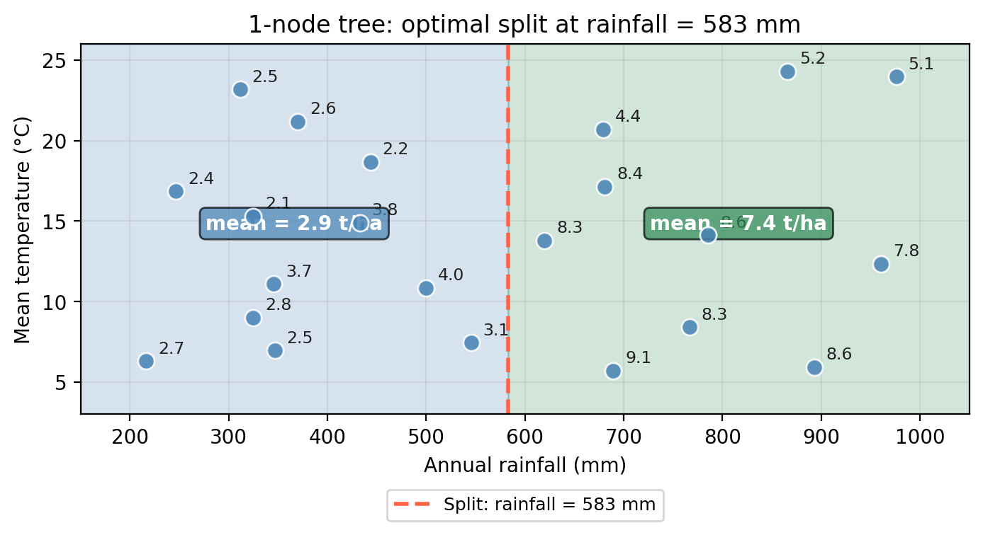
The root node split
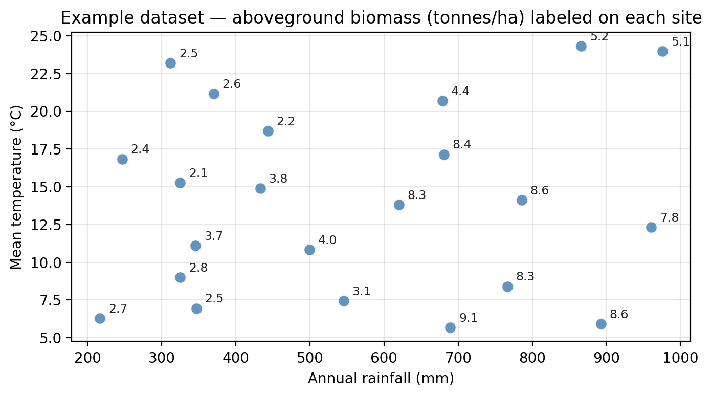
In regression trees, the predicted value at the leaf is the mean of all training observations that reach this leaf.
We begin with our full training dataset:
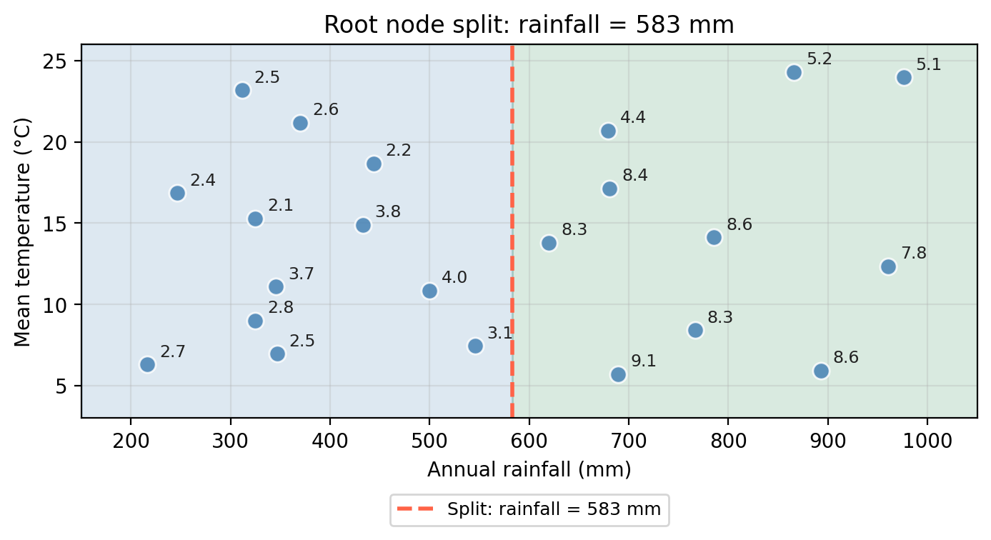
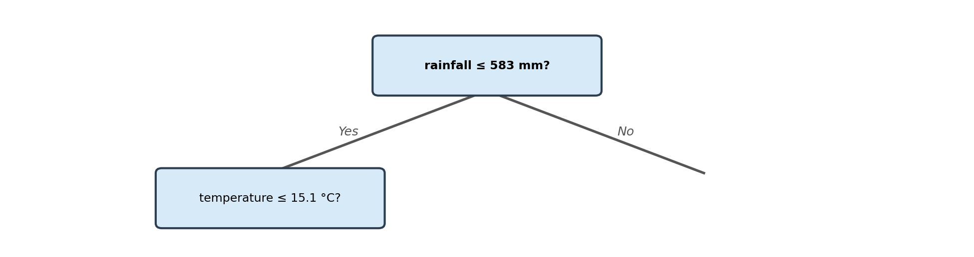
The root node split
The root node asks whether rainfall ≤ 583mm" mm. This creates a vertical division in the predictor space.
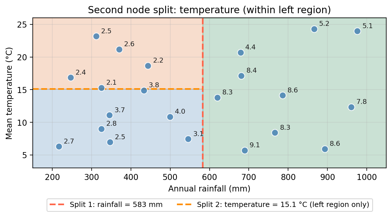
The second split
The second node looks at observations in the left region (rainfall ≤ 583 mm) and asks whether temperature ≤ 15.1 °C. This adds a horizontal split within that region only.
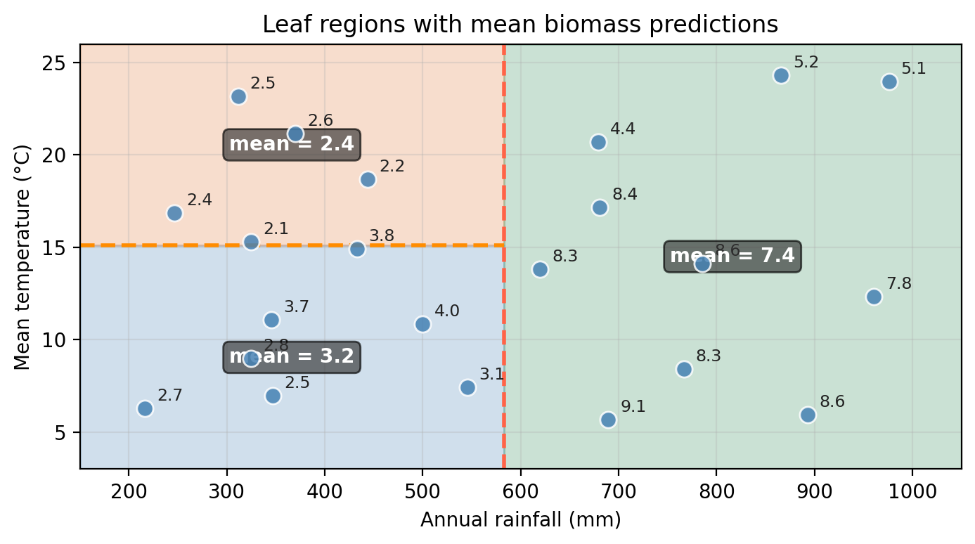
Leaf regions and predictions
Leaves correspond to the final regions in the predictor space.
Each observation is assigned the mean response of the training observations that fall in the same region:
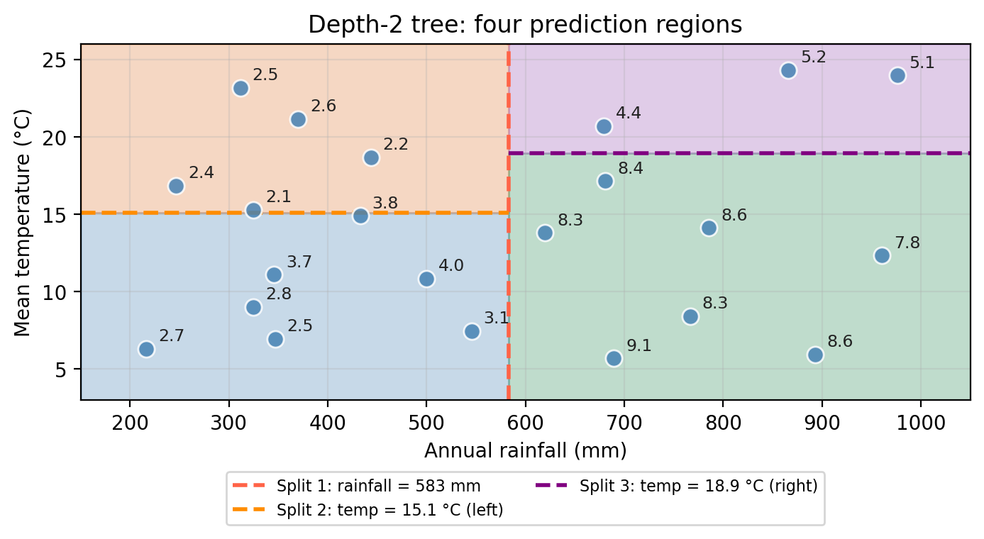
Check-in
The plot shows a new split added to the right region.
Modify the tree diagram to include a node and leaves that represent this additional split.
Regression tree: summary
A regression tree works by:
1. Dividing the predictor space — the set of all possible values for \(X_1, X_2, \ldots, X_p\) — into \(J\) non-overlapping rectangular regions \(R_1, R_2, \ldots, R_J\).
2. Assigning a prediction to each region: for every observation that falls into region \(R_j\), the prediction is the mean response of the training observations in \(R_j\).
Fitting a regression tree
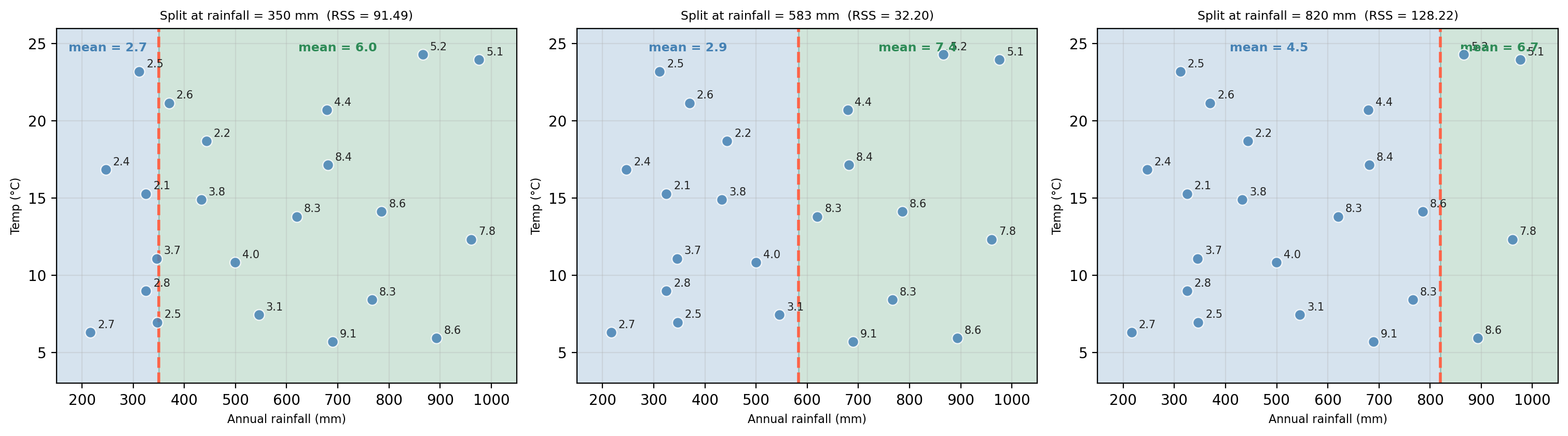
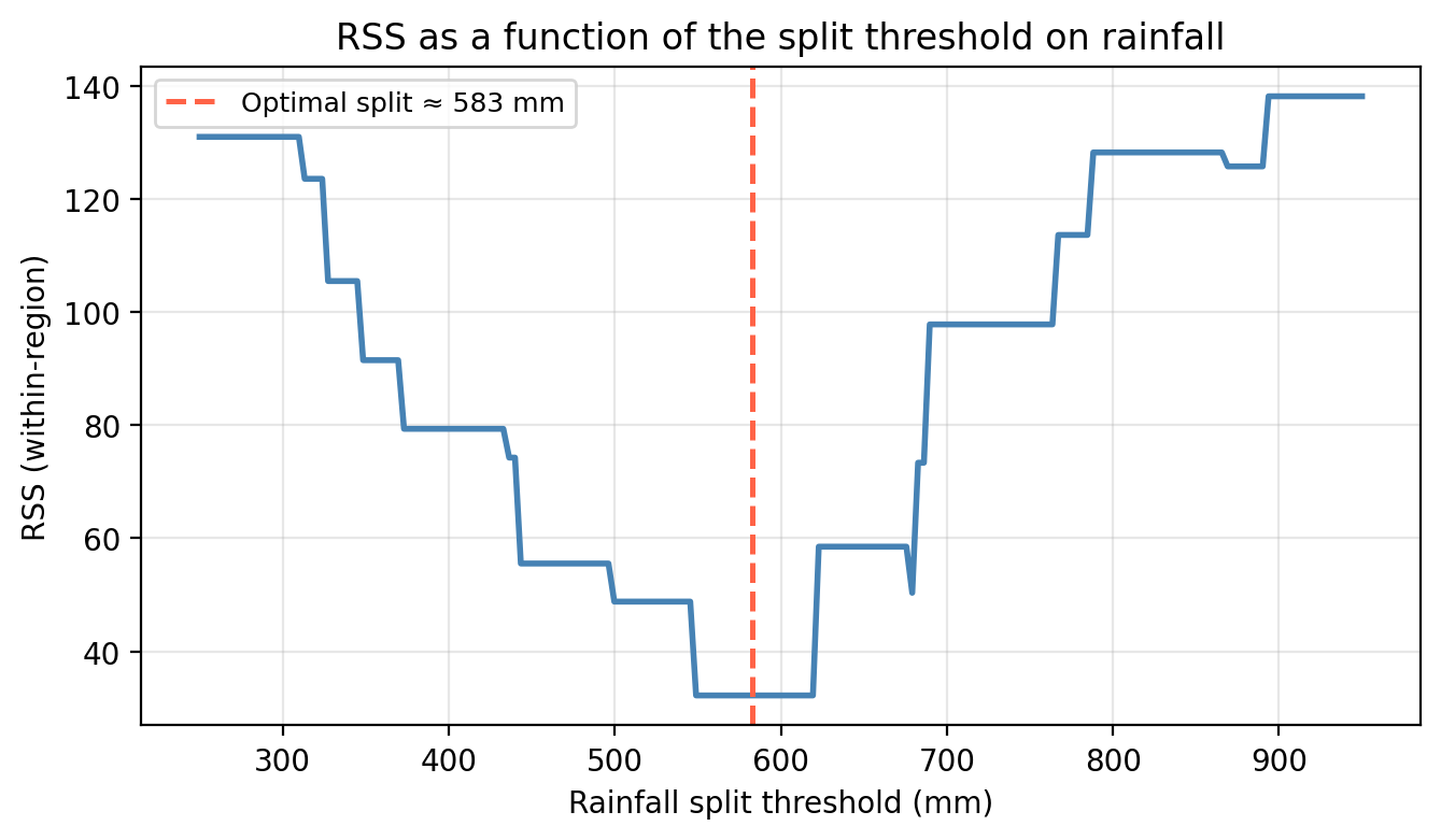
Finding the first split
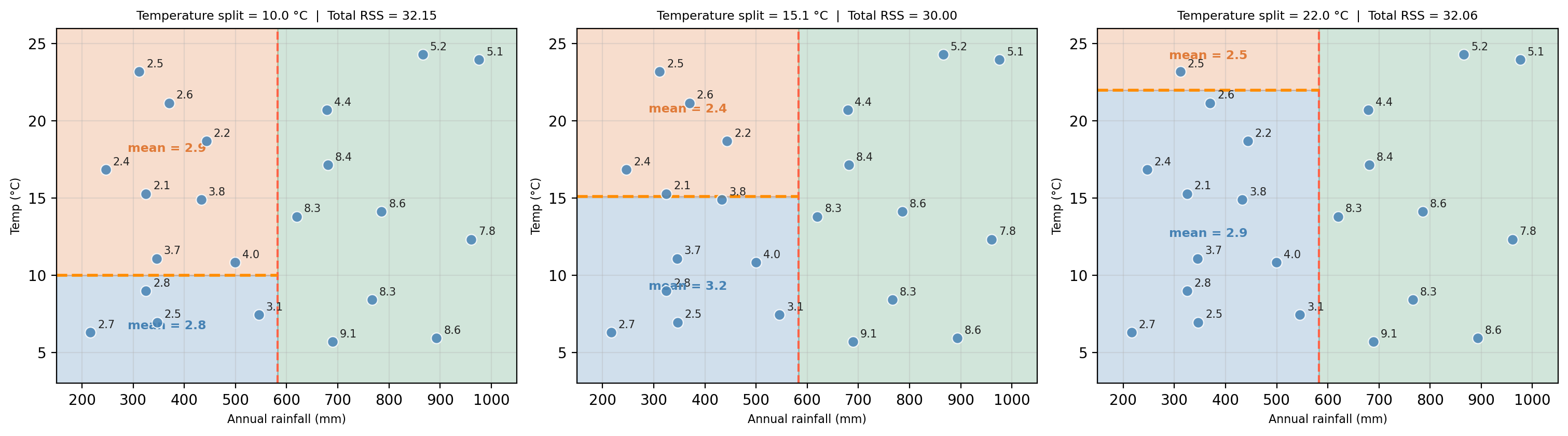
The algorithm evaluates every possible threshold on every predictor. Here are three candidate splits on rainfall:
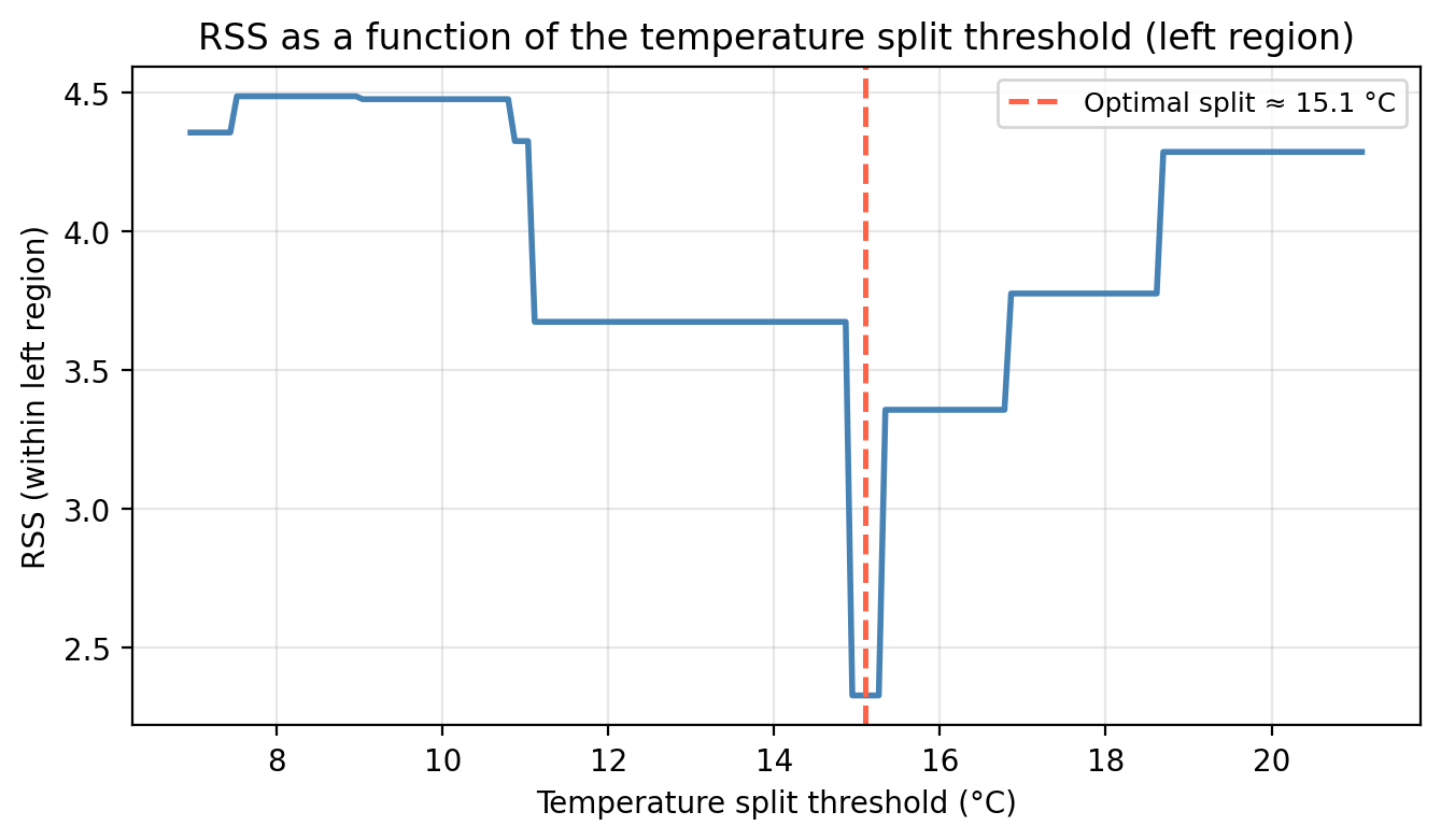
Finding the second split
After the first split, the algorithm considers splitting each resulting region. Here are three candidate temperature splits within the left (low-rainfall) region:
Overfitting in decision trees
A fully-grown decision tree will perfectly fit the training data but generalize poorly to new observations.
As the tree grows deeper, the decision boundaries become increasingly specific to the training data:
Go to website for images
Check-in
The full tree has a training MSE of 0. What does this tell us about how well it fits the training data?
Would you expect the full tree to perform better or worse than the depth-3 tree on new, unseen data? Why?
What are two approaches you could use to control the complexity of a decision tree?
A training MSE near zero means the full tree essentially memorizes the training data — every observation is in its own leaf.
The full tree would likely perform worse on new data. It has memorized noise in the training set (high variance) rather than learning the underlying pattern.
Two common approaches:
- Maximum depth: limit how many levels the tree can grow
- Minimum samples per leaf: stop splitting when a region has too few observations
Controlling tree complexity
Maximum depth and minimum samples per leaf are both hyperparameters that control the complexity vs. fit tradeoff:
- A shallower tree has fewer, larger regions
- A deeper tree has more, smaller regions
How would cross-validation be applied to find the best values for these hyperparameters?
Compute the CV-MSE for a grid of depth and samples-per-leaf values. Select the combination that gives the lowest cross-validation error as the hyperparameters for the final tree.
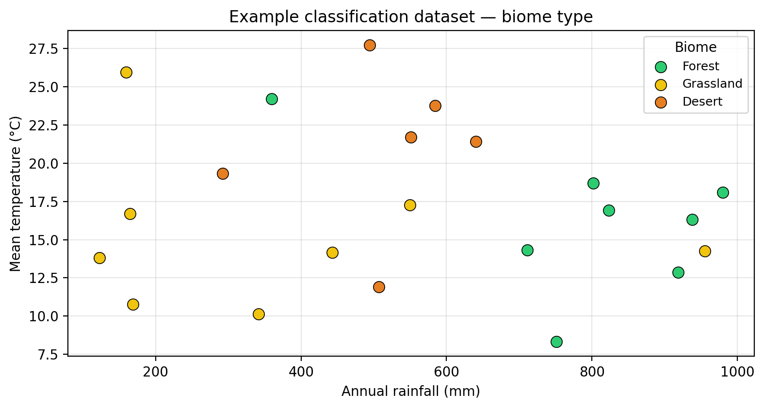
A classification dataset
The same 22 sites, same predictors (rainfall, temperature), but a categorical response: the site’s biome type:
What is a classification tree?
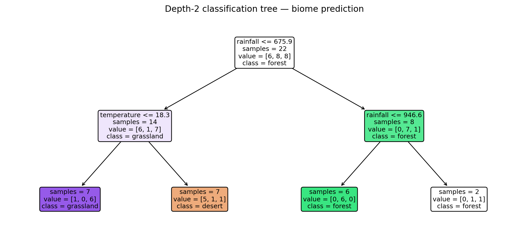
A classification tree has the same structure as a regression tree (root, internal nodes, branches, and leaves) but makes categorical predictions instead of numerical ones.
For each leaf node, the prediction is the majority class (most common class) among the training observations that reach that leaf.
Check-in
Use the classification tree to predict the biome type for a new site with rainfall = 500 mm and temperature = 15°C.
Check-in
Use the classification tree to predict the biome type for a new site with rainfall = 500 mm and temperature = 15°C.
- Root: Is rainfall 500 mm ≤ 675.9 mm? Yes → left branch (low rainfall)
- Internal node: Is temperature 15°C ≤ 18.3°C? Yes → left branch (low temperature)
- Leaf: The majority class in this leaf is grassland
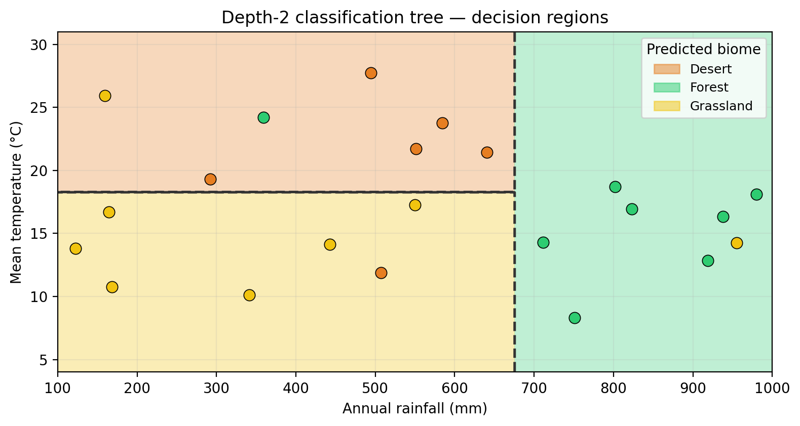
Decision regions
Just like regression trees, classification trees divide the predictor space into rectangular regions:
Fitting a classification tree
Fitting a classification tree
A classification tree is fitted by:
1. Dividing the predictor space into \(J\) non-overlapping regions \(R_1, \ldots, R_J\).
2. Predicting the majority class among training observations in each region \(R_j\). . . .
As with regression trees, recursive binary splitting is used, but we cannot use RSS for classification. Instead, we measure the impurity of the resulting regions.
We are often interested in the class proportions at each leaf, not just the predicted class. These give a sense of prediction confidence or purity: a leaf where 95% of observations share one class is more reliable than a 60/40 split.
Check-in
Looking at the classification tree, which leaf has the most confident predictions? Which would you say is the most “pure” and why?
Check-in
The forest leaf (leftmost, green). All training observations in that region belong to the same class — forest — so the predicted class proportion is 1.0 for forest and 0.0 for all others.
The tree is maximally confident there: no ambiguity in the prediction.
In contrast, the other leaves contain a mix of classes, making their predictions less reliable.
Gini impurity
The most common splitting criterion for classification trees is the Gini impurity index: a measure of how mixed the classes are in a given region.
- A region where all observations belong to the same class → Gini impurity = 0 (perfectly pure)
- The more evenly observations are spread across classes → higher impurity
At each step, recursive binary splitting searches for the variable and threshold that produce the purest child regions.
Entropy is another common impurity measure that behaves similarly and tends to produce very similar trees in practice.
Trees vs. linear models
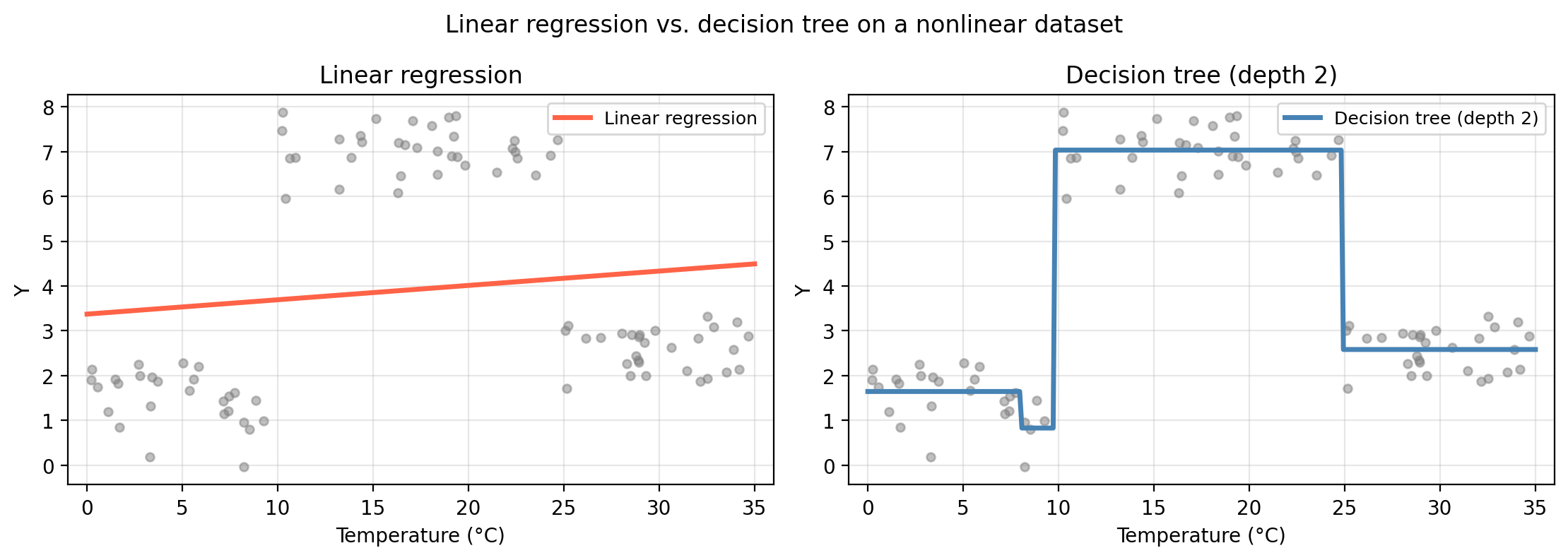
Decision trees and linear models capture fundamentally different types of relationships:
- Linear models (regression, ridge, lasso): assume the response changes smoothly and approximately linearly with the predictors
- Decision trees: make no such assumption, they partition the predictor space into rectangular regions with constant predictions
Trees naturally capture nonlinear, step-like relationships that linear models cannot fit well.
Linear models perform better when the true relationship is approximately linear and smooth.
Trees vs. linear models: example
Synthetic data where Y depends on temperature in a step-function pattern:
Trees vs. linear models: summary
| Interpretability |
High, easy to visualize |
Ok, coefficients interpretable |
| Nonlinear relationships |
Handles them naturally |
Requires feature engineering |
| Prediction accuracy |
Often lower |
Competitive when relationship is linear |
| Variance |
High, sensitive to small changes |
Generally lower |
| Variable selection |
Implicit (splits on useful variables) |
Requires explicit methods (e.g., lasso) |