Lab 6: Decision Trees

Download the Lab Template

Download the lab template here and move to your eds232-labs repository.

Background

In this lab you’ll build and tune a decision tree to predict forest cover type from wilderness cartographic data. This is a multi-class classification problem used by the US Forest Service to map land cover without costly field surveys.

Dataset: UCI Forest Cover Type (id=31). 581,012 records from four wilderness areas in the Roosevelt National Forest, Colorado. Features include elevation, slope, hillshade, distance to water and roads, wilderness area, and soil type. Our response variable, Cover_Type, includes 7 different forest types: Spruce/Fir, Lodgepole Pine, Ponderosa Pine, Cottonwood/Willow, Aspen, Douglas-fir, Krummholz (encoded as integers from 1 to 7). More information on the data can be found here.

Step 1: Load and Explore the Data

Code

import pandas as pd
import numpy as np
import matplotlib.pyplot as plt
from ucimlrepo import fetch_ucirepo
from sklearn.model_selection import train_test_split, cross_val_score, GridSearchCV
from sklearn.tree import DecisionTreeClassifier, plot_tree
from sklearn.metrics import accuracy_score

Code

forest = fetch_ucirepo(id=31)

df = pd.concat([forest.data.features, forest.data.targets], axis=1)

print(f"Full dataset shape: {df.shape}")
print()
print("Cover type distribution (full dataset):")
print(df['Cover_Type'].value_counts().sort_index())
df.head()

Full dataset shape: (581012, 55)

Cover type distribution (full dataset):
Cover_Type
1    211840
2    283301
3     35754
4      2747
5      9493
6     17367
7     20510
Name: count, dtype: int64

	Elevation	Aspect	Slope	Horizontal_Distance_To_Hydrology	Vertical_Distance_To_Hydrology	Horizontal_Distance_To_Roadways	Hillshade_9am	Hillshade_Noon	Hillshade_3pm	Horizontal_Distance_To_Fire_Points	...	Cover_Type
0	2596	51	3	258	0	510	221	232	148	6279	...	5
1	2590	56	2	212	-6	390	220	235	151	6225	...	5
2	2804	139	9	268	65	3180	234	238	135	6121	...	2
3	2785	155	18	242	118	3090	238	238	122	6211	...	2
4	2595	45	2	153	-1	391	220	234	150	6172	...	5

5 rows × 55 columns

Step 2: Preprocess

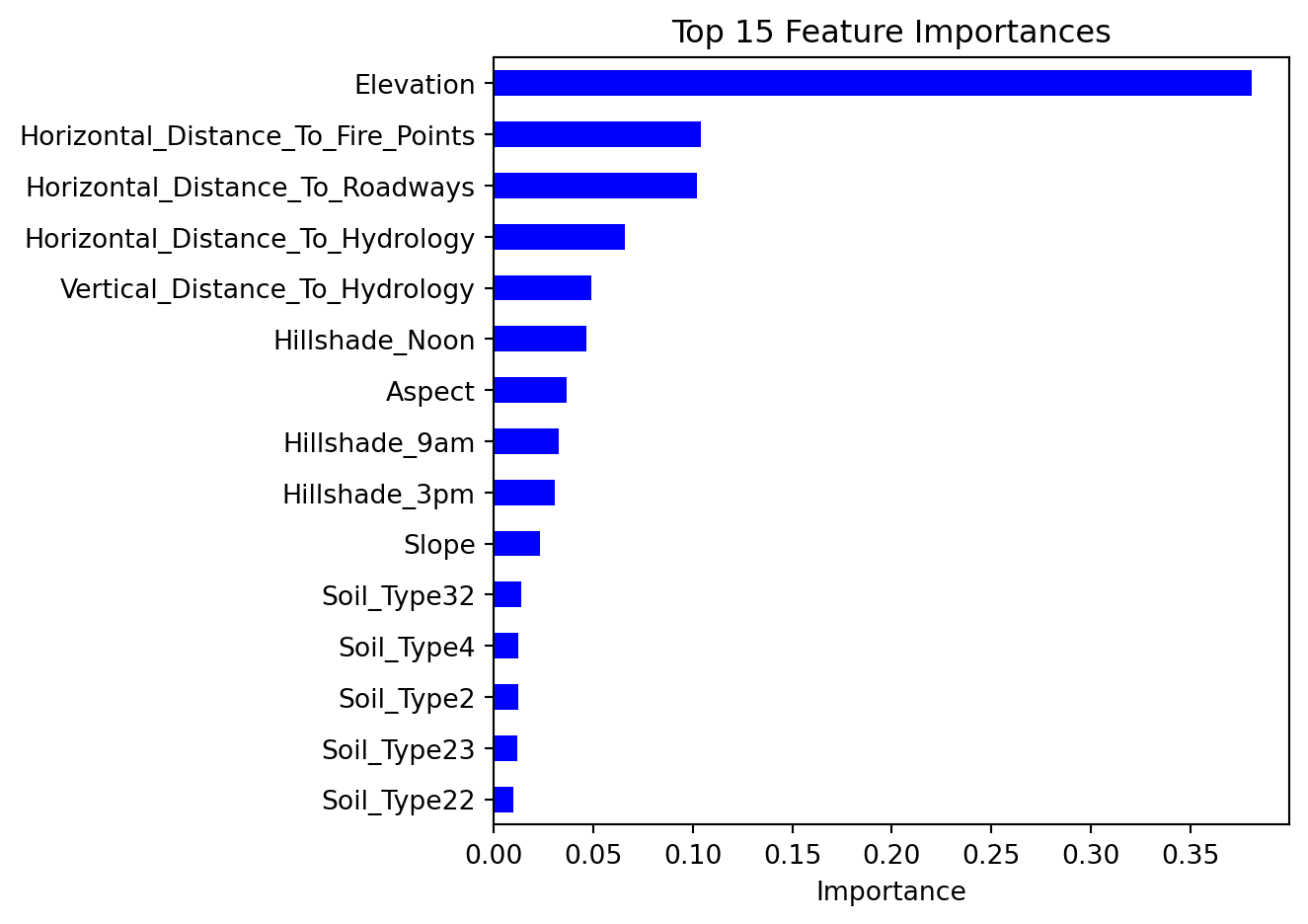
The Forest Cover Type dataset is already clean and fully numeric, meaning all features are encoded as integers. The 54 features include:

10 continuous: elevation, aspect, slope, hillshade indices, distances to hydrology, roadways, and fire points
44 binary: 4 wilderness area indicators and 40 soil type indicators

No encoding or scaling is needed. We will sample 30,000 rows to keep lab runtimes manageable.

Code

df_sample = df.sample(n=30_000, random_state=42)

features = [c for c in df_sample.columns if c != 'Cover_Type']
X = df_sample[features]
y = df_sample['Cover_Type']

Code

X_train, X_test, y_train, y_test = train_test_split(X, y, test_size=0.3,stratify=y, random_state=42)
print(f"Training samples: {len(X_train):,}  |  Test samples: {len(X_test):,}")

Training samples: 21,000  |  Test samples: 9,000

Step 3: Fit a Decision Tree

To start, we will fit a decision tree without specifying any hyperparameters.

Code

dt_full = DecisionTreeClassifier(random_state=42)
dt_full.fit(X_train, y_train)

train_acc = accuracy_score(y_train, dt_full.predict(X_train))
test_acc  = accuracy_score(y_test,  dt_full.predict(X_test))

print(f"Untuned tree depth:  {dt_full.get_depth()}")
print(f"Training accuracy:         {train_acc:.3f}")
print(f"Test accuracy:             {test_acc:.3f}")

Untuned tree depth:  35
Training accuracy:         1.000
Test accuracy:             0.780

Uh oh! Look at the difference between our test accuracy and our training accuracy. It looks like our model is overfitting! Let’s try tuning to prevent this.

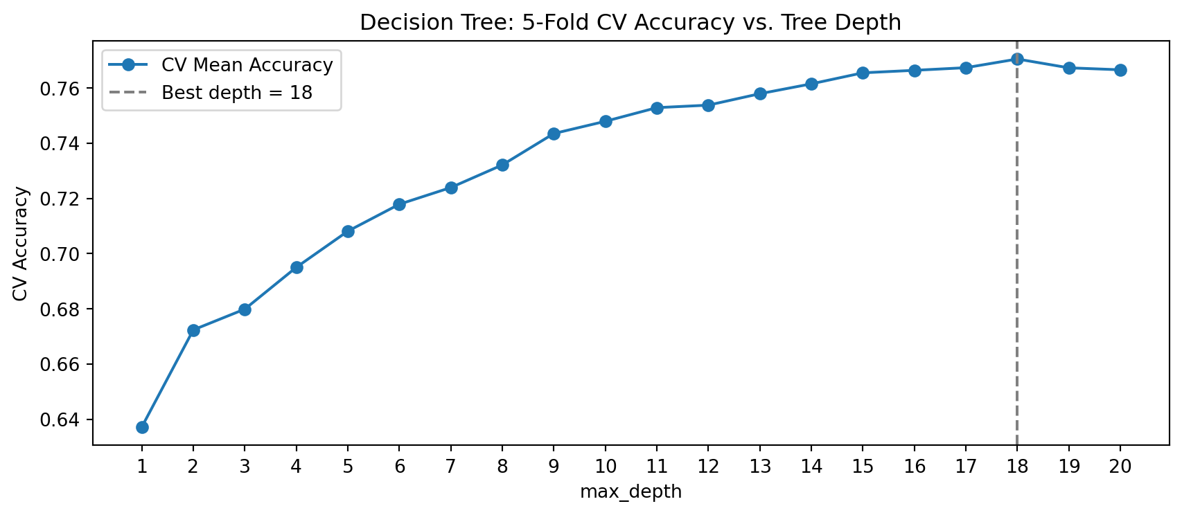
Step 4: Tune `max_depth` with Cross-Validation

Rather than evaluating each depth on the held-out test set (which leaks information), we use 5-fold cross-validation on the training data. We will first tune max_depth, a hyperparameter which limits how many levels a tree can grow. Perform cross fold validation, iterating over a max depth from 1 to 20.

Code

depths = range(1, 21)
cv_means =  []

for depth in depths:
    dt = DecisionTreeClassifier(max_depth=depth, random_state=42)
    scores = cross_val_score(dt, X_train, y_train, cv=5, scoring='accuracy')
    cv_means.append(scores.mean())

cv_means = np.array(cv_means)
best_depth = list(depths)[np.argmax(cv_means)]
print(f"Best max_depth (5-fold CV): {best_depth}  (CV accuracy: {cv_means.max():.3f})")

plt.figure(figsize=(9, 4))
plt.plot(list(depths), cv_means, label='CV Mean Accuracy', marker='o')
plt.axvline(best_depth, color='gray', linestyle='--', label=f'Best depth = {best_depth}')
plt.xlabel('max_depth')
plt.ylabel('CV Accuracy')
plt.xticks(list(depths))
plt.title('Decision Tree: 5-Fold CV Accuracy vs. Tree Depth')
plt.legend()
plt.tight_layout()
plt.show()

Best max_depth (5-fold CV): 18  (CV accuracy: 0.771)

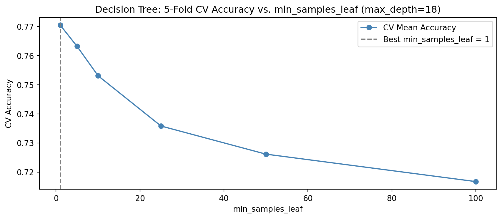
Step 5: Tune `min_samples_leaf` with Cross-Validation

min_samples_leaf sets the minimum number of training samples required at any leaf node. Perform cross fold validation, iterating over the following numbers of minimum samples: 1, 5, 10, 25, 50, and 100.

Code

leaf_sizes = [1, 5, 10, 25, 50, 100]
leaf_cv_means = []

for n in leaf_sizes:
    dt = DecisionTreeClassifier(max_depth=best_depth, min_samples_leaf=n, random_state=42)
    scores = cross_val_score(dt, X_train, y_train, cv=5, scoring='accuracy')
    leaf_cv_means.append(scores.mean())


leaf_cv_means = np.array(leaf_cv_means)

best_leaf = leaf_sizes[np.argmax(leaf_cv_means)]
print(f"Best min_samples_leaf (5-fold CV): {best_leaf}  (CV accuracy: {leaf_cv_means.max():.3f})")

plt.figure(figsize=(9, 4))
plt.plot(leaf_sizes, leaf_cv_means, label='CV Mean Accuracy', marker='o', color='steelblue')
plt.axvline(best_leaf, color='gray', linestyle='--', label=f'Best min_samples_leaf = {best_leaf}')
plt.xlabel('min_samples_leaf')
plt.ylabel('CV Accuracy')
plt.title(f'Decision Tree: 5-Fold CV Accuracy vs. min_samples_leaf (max_depth={best_depth})')
plt.legend()
plt.tight_layout()
plt.show()

Best min_samples_leaf (5-fold CV): 1  (CV accuracy: 0.771)

Discuss with a partner what it means to have a higher min_samples_leaf value.

Step 6: Joint Tuning with `GridSearchCV`

Tuning hyperparameters one at a time ignores their interactions. GridSearchCV evaluates every combination in a parameter grid using cross-validation, finding the jointly optimal settings. Use the max_depth values of 5, 10, 15, 16, 17,18, 19 20, the min_samples_leaf values of 1, 5, 10, and 25, and the criterion options of gini and entropy to find the best combination of parameters.

Code

param_grid = {
    'max_depth':        [5, 10, 15, 16, 17,18, 19, 20],
    'min_samples_leaf': [1, 5, 10, 25],
    'criterion':        ['gini', 'entropy']
}

grid_search = GridSearchCV(
    DecisionTreeClassifier(random_state=42),
    param_grid,
    cv=5,
    scoring='accuracy',
    n_jobs=-1
)
grid_search.fit(X_train, y_train)

print(f"Best parameters:  {grid_search.best_params_}")

dt_best = grid_search.best_estimator_
dt_acc  = accuracy_score(y_test, dt_best.predict(X_test))
print(f"Test accuracy:    {dt_acc:.3f}")

Best parameters:  {'criterion': 'gini', 'max_depth': 18, 'min_samples_leaf': 1}
Test accuracy:    0.776

Does the best max_depth and min_samples_leaf from GridSearchCV match what you found by tuning it individually in Step 4? If not, why might joint tuning arrive at a different answer?

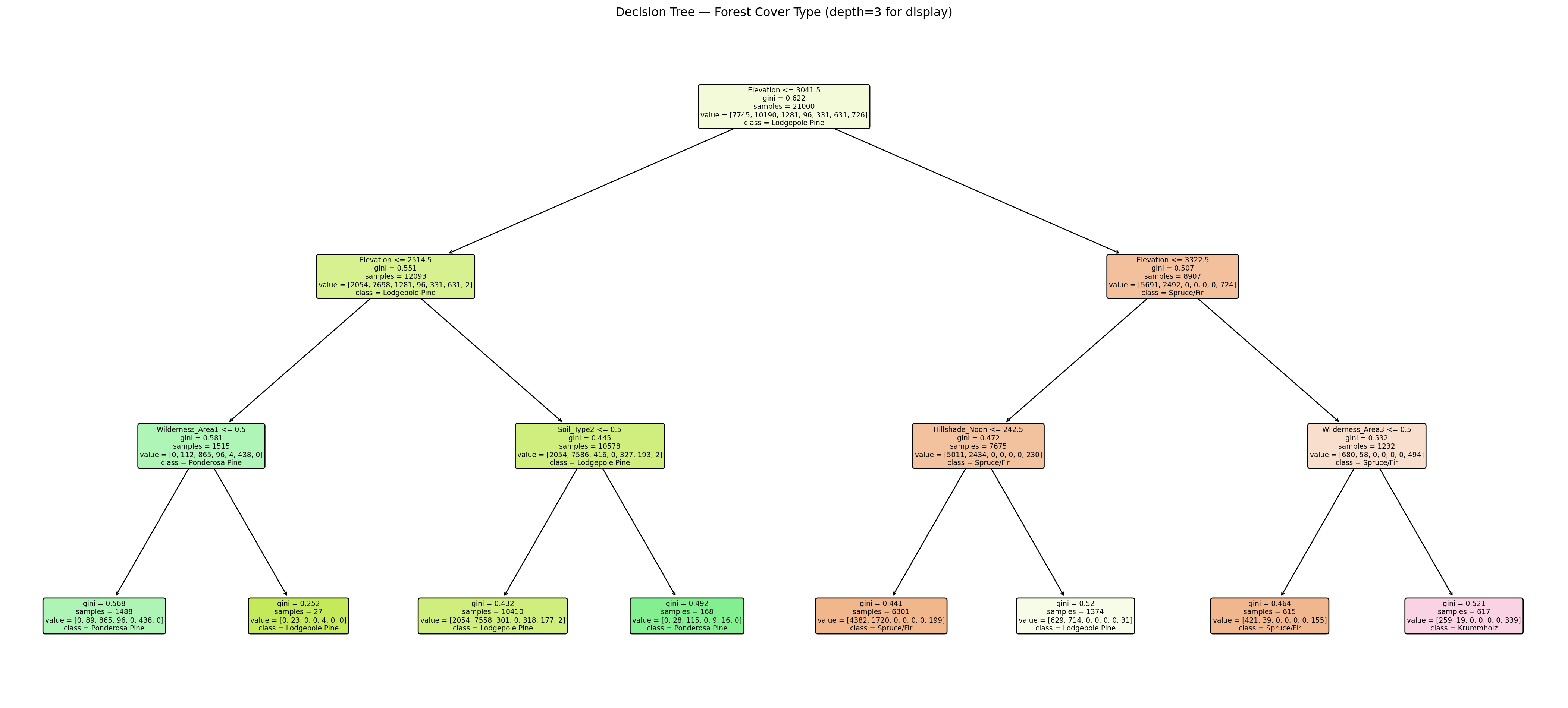
Step 7: Visualize the Best Tree

Create a visualization of your decision tree with a max_depth of 3 (for plotting purposes), and the values that your grid search found to be best for min_samples_leaf and criterion.

Review the value counts of our y_train here

Code

print("Cover type distribution (training set):")
print(y_train.value_counts().sort_index())

Cover type distribution (training set):
Cover_Type
1     7745
2    10190
3     1281
4       96
5      331
6      631
7      726
Name: count, dtype: int64

Code

dt_viz = DecisionTreeClassifier(
    max_depth=3,
    min_samples_leaf=grid_search.best_params_['min_samples_leaf'],
    criterion=grid_search.best_params_['criterion'],
    random_state=42
)
dt_viz.fit(X_train, y_train)

plt.figure(figsize=(22, 10))
class_names = ['Spruce/Fir', 'Lodgepole Pine', 'Ponderosa Pine',
               'Cottonwood/Willow', 'Aspen', 'Douglas-fir', 'Krummholz']

plot_tree(dt_viz, feature_names=features, class_names=class_names,
          filled=True, rounded=True, fontsize=7)

plt.title('Decision Tree — Forest Cover Type (depth=3 for display)')
plt.tight_layout()
plt.show()

Discussion Questions:

What feature appears at the root node (the very first split)? Does it make ecological sense that this feature is the most informative for separating forest cover types?

Look at the elevation threshold used at the root split (in meters). Rocky Mountain subalpine forests typically begin around 2,750–3,000m. Does the split value align with a meaningful ecological boundary?

Look at the observation below. What Forest Cover type would this observation be classified as with our tree above?

Elevation                             2006
Aspect                                  53
Slope                                   12
Horizontal_Distance_To_Hydrology         0
Vertical_Distance_To_Hydrology           0
Horizontal_Distance_To_Roadways        255
Horizontal_Distance_To_Roadways        255
Hillshade_9am                          227
Hillshade_Noon                         215
Hillshade_3pm                          120
Horizontal_Distance_To_Fire_Points     366
Wilderness_Area1                         0
Cover_Type                               4
Name: 2067, dtype: int64

#	Cover Type
1	Spruce/Fir
2	Lodgepole Pine
3	Ponderosa Pine
4	Cottonwood/Willow
5	Aspen
6	Douglas-fir
7	Krummholz

Step 8: Feature Importance

With 54 features, many soil type indicators will have very little importance. Create a plot showing the top 15 most important features.

Code

feat_imp = pd.Series(dt_best.feature_importances_, index=features).sort_values(ascending=False)

plt.figure(figsize=(7, 5))
feat_imp.head(15).sort_values().plot(kind='barh', color='blue')
plt.xlabel('Importance')
plt.title('Top 15 Feature Importances')
plt.tight_layout()
plt.show()

Which feature is most important? Is this the same feature that appeared at the root node of the tree in Step 7?

Background

Step 1: Load and Explore the Data

Step 2: Preprocess

Step 3: Fit a Decision Tree

Uh oh! Look at the difference between our test accuracy and our training accuracy. It looks like our model is overfitting! Let’s try tuning to prevent this.

Step 4: Tune max_depth with Cross-Validation

Step 5: Tune min_samples_leaf with Cross-Validation

Step 6: Joint Tuning with GridSearchCV

Step 7: Visualize the Best Tree

Step 8: Feature Importance

Step 4: Tune `max_depth` with Cross-Validation

Step 5: Tune `min_samples_leaf` with Cross-Validation

Step 6: Joint Tuning with `GridSearchCV`