Download the lab template here and move to your eds232-labs repository.
Background
Dataset: UCI Forest Cover Type (id=31) (the same dataset from Lab 6)
In Lab 6, you found that a single decision tree can achieve strong performance on forest cover classification but tends to overfit. In this lab you will apply three ensemble methods that address this problem in different ways:
Method
Strategy
Bagging
Average many trees trained on bootstrap samples
Random Forest
Bagging + random feature subsets at each split
Gradient Boosting
Build trees sequentially, each correcting the previous
forest = fetch_ucirepo(id=31)df = pd.concat([forest.data.features, forest.data.targets], axis=1)print(f"Full dataset shape: {df.shape}")print()print("Cover type distribution (full dataset):")print(df['Cover_Type'].value_counts().sort_index())df.head()
Full dataset shape: (581012, 55)

Cover type distribution (full dataset):
Cover_Type
1    211840
2    283301
3     35754
4      2747
5      9493
6     17367
7     20510
Name: count, dtype: int64
Elevation
Aspect
Slope
Horizontal_Distance_To_Hydrology
Vertical_Distance_To_Hydrology
Horizontal_Distance_To_Roadways
Hillshade_9am
Hillshade_Noon
Hillshade_3pm
Horizontal_Distance_To_Fire_Points
...
Soil_Type35
Soil_Type36
Soil_Type37
Soil_Type38
Soil_Type39
Soil_Type40
Wilderness_Area2
Wilderness_Area3
Wilderness_Area4
Cover_Type
0
2596
51
3
258
0
510
221
232
148
6279
...
0
0
0
0
0
0
0
0
0
5
1
2590
56
2
212
-6
390
220
235
151
6225
...
0
0
0
0
0
0
0
0
0
5
2
2804
139
9
268
65
3180
234
238
135
6121
...
0
0
0
0
0
0
0
0
0
2
3
2785
155
18
242
118
3090
238
238
122
6211
...
0
0
0
0
0
0
0
0
0
2
4
2595
45
2
153
-1
391
220
234
150
6172
...
0
0
0
0
0
0
0
0
0
5
5 rows × 55 columns
Step 2: Repeat Preprocessing Steps from Lab 6
Code
df_sample = df.sample(n=30_000, random_state=42)features = [c for c in df_sample.columns if c !='Cover_Type']X = df_sample[features]y = df_sample['Cover_Type']X_train, X_test, y_train, y_test = train_test_split(X, y, test_size=0.33, random_state=42)print(f"Training samples: {len(X_train):,} | Test samples: {len(X_test):,}")
Training samples: 20,100 | Test samples: 9,900
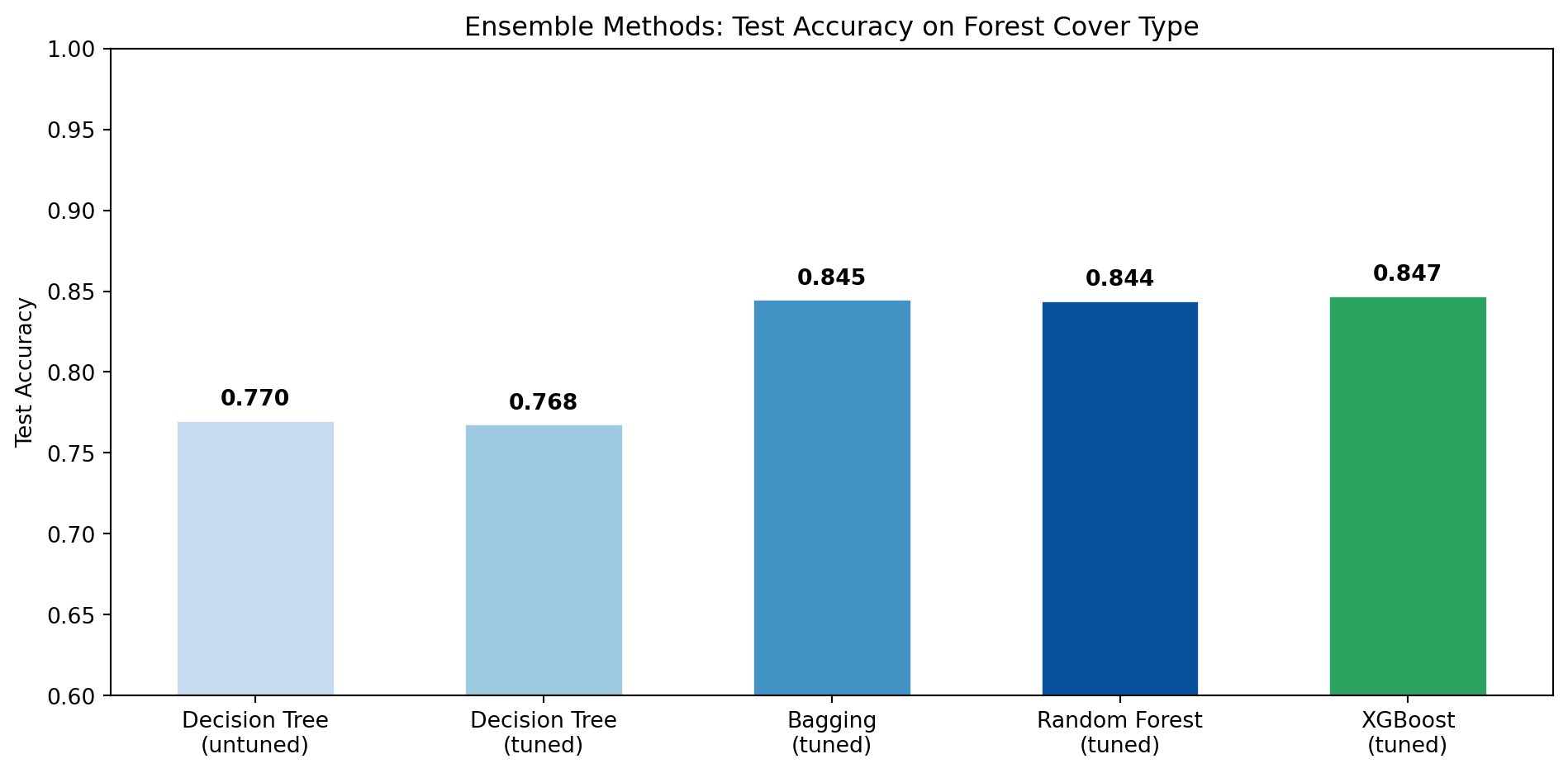
Step 3: Decision Tree Baseline
Re-run the both the untuned and tuned decision tree we fit in Lab 6.
dt_tuned = DecisionTreeClassifier(criterion='entropy', max_depth=20, min_samples_leaf=1, random_state=42)dt_tuned.fit(X_train, y_train)dt_tuned_train_acc = accuracy_score(y_train, dt_tuned.predict(X_train))dt_tuned_test_acc = accuracy_score(y_test, dt_tuned.predict(X_test))print("Untuned Decision Tree Metrics:")print(f"Decision Tree depth: {dt.get_depth()}")print(f"Decision Tree training acc: {dt_train_acc:.3f}")print(f"Decision Tree test acc: {dt_test_acc:.3f}")print()print("Tuned Decision Tree Metrics")print(f"Tuned Decision Tree depth: {dt_tuned.get_depth()}")print(f"Tuned Decision Tree test acc: {dt_tuned_test_acc:.3f}")
Untuned Decision Tree Metrics:
Decision Tree depth:          35
Decision Tree training acc:   1.000
Decision Tree test acc:  0.770

Tuned Decision Tree Metrics
Tuned Decision Tree depth:        20
Tuned Decision Tree test acc:     0.768
Recall from Lab 6: The gap between training and test accuracy is a clear sign of overfitting. A fully-grown tree memorizes the training set. Ensemble methods are designed to close this gap.
Background: Bagging
The variance problem: Decision trees suffer from high variance where small changes in training data can produce very different trees and predictions. A general strategy to reduce variance is to fit many models on different datasets and average their predictions. The challenge is that we typically only have one dataset. Bagging (Bootstrap Aggregation) solves this.
Bootstrap Aggregation
Bagging generates many training sets from a single dataset by bootstrapping (sampling with replacement) so each bootstrap sample is the same size as the original, but some observations repeat and others are left out. Then:
Fit a separate decision tree on each of the B bootstrapped training sets
For a new observation, obtain B predictions
Regression: Average all B predictions → \(\hat{f}_{bag}(x) = \frac{1}{B}\sum_{b=1}^{B}\hat{f}^{*b}(x)\)
Classification: Take a majority vote across all B predictions
Unlike tuning tree depth, choosing a larger B never causes overfitting, but it does add compute time. Select B large enough that the out-of-bag error stabilizes.
Out-of-Bag (OOB) Error
Roughly one-third of observations are excluded from any given bootstrap sample, known as the out-of-bag (OOB) observations. Each observation can be predicted using only the trees that were not trained on it, providing a free estimate of test error without cross-validation. OOB error is a valid estimate of generalization performance because each prediction is made by trees that never saw that observation during training.
Step 4: Fit a Bagging Classifier
Fit a BaggingClassifier with n_estimators=50 and oob_score=True. The out-of-bag (OOB) score is a free estimate of test accuracy computed from the bootstrap samples left out of each tree. Compare OOB score, training accuracy, and test accuracy to the single decision tree.
Code
bag = BaggingClassifier(n_estimators=50, oob_score=True, random_state=42, n_jobs=-1)bag.fit(X_train, y_train)bag_train_acc = accuracy_score(y_train, bag.predict(X_train))bag_test_acc = accuracy_score(y_test, bag.predict(X_test))print(f"Bagging OOB score: {bag.oob_score_:.3f}")print(f"Bagging training acc: {bag_train_acc:.3f}")print(f"Bagging test acc: {bag_test_acc:.3f}")
Bagging OOB score:            0.838
Bagging training acc:         1.000
Bagging test acc:             0.840
How does the OOB score compare to test accuracy? How did bagging change the gap between training and test accuracy relative to the single decision tree?
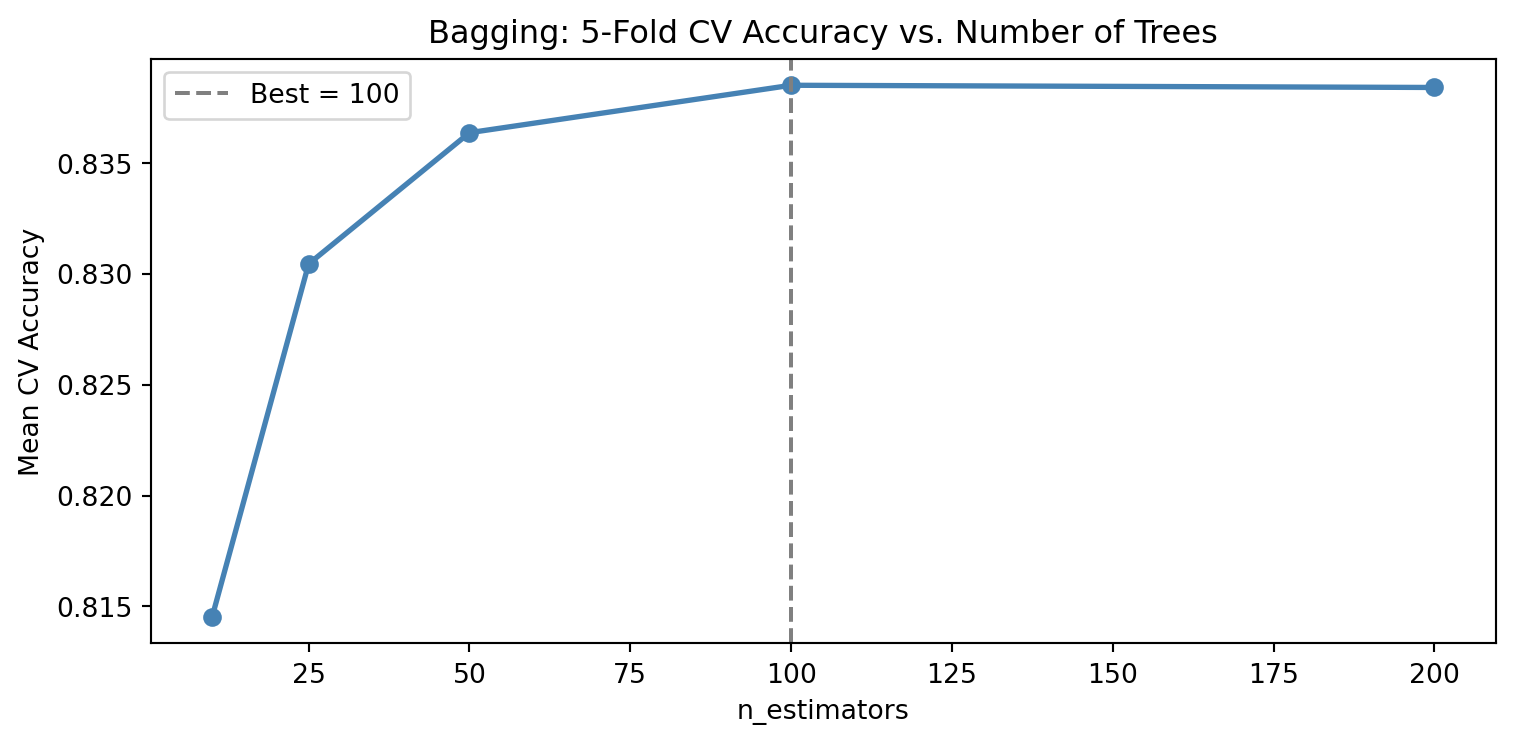
Step 5: Tune the Number of Trees for Bagging
More trees in a bagging model generally improve performance up to a point, after which the gains plateau. Unlike boosting, adding trees in bagging never hurts but it does add compute time. Use 5-fold cross-validation on the training set to evaluate n_estimators values of 10, 25, 50, 100, and 200. Plot CV accuracy vs. number of trees.
How do we pick the number of estimators to include in hyperparameter tuning? Refer to the table below for applications across different fields:
At what point do additional trees stop providing meaningful improvement? How does this differ from what you would expect with decision trees, where not specifying a max_depth can cause overfitting?
Background: Random Forests
Random forests extend bagging by decorrelating the trees. At every split, only a random subset of m < p predictors is considered as split candidates.
Default values:
Classification: \(m = \sqrt{p}\)
Regression: \(m = p/3\)
Why Decorrelation Matters
When one predictor strongly associates with the response, nearly every bagged tree places it at the top split, producing trees that are highly correlated with each other. Averaging correlated predictions reduces variance less effectively than averaging uncorrelated ones. By restricting which predictors are available at each split, random forests break this dominance and force diversity among trees — further reducing variance beyond what bagging alone achieves.
When \(m = p\) (all predictors available at every split), random forests reduce exactly to bagging.
Tuning m (max_features)
Smaller m introduces more randomness, producing less-correlated trees with lower variance but potentially higher bias. Cross-validation can be used to find the optimal m when performance is sensitive to this choice. Random forests outperform bagging most when one or a few predictors dominate the response since restricting splits prevents those predictors from monopolizing every tree.
Step 6: Fit a Random Forest
Fit a RandomForestClassifier using the best n_estimators found in Step 5 and the default max_features='sqrt'. Enable oob_score=True. Compare test accuracy and OOB score to bagging and the single tree.
Code
rf = RandomForestClassifier( n_estimators=best_n_bag, max_features='sqrt', oob_score=True, random_state=42, n_jobs=-1)rf.fit(X_train, y_train)rf_train_acc = accuracy_score(y_train, rf.predict(X_train))rf_test_acc = accuracy_score(y_test, rf.predict(X_test))print(f"Decision Tree test acc: {dt_test_acc:.3f}")print(f"Bagging test acc: {bag_test_acc:.3f}")print()print(f"Random Forest OOB score: {rf.oob_score_:.3f}")print(f"Random Forest test acc: {rf_test_acc:.3f}")
Decision Tree test acc:   0.770
Bagging test acc:         0.845

Random Forest OOB score:  0.838
Random Forest test acc:   0.837
Step 7: Tune the Random Forest with GridSearchCV
Tuning max_features alone ignores interactions with tree depth. Use GridSearchCV to jointly search over:
n_estimators: [50, 100]
max_features: ['sqrt', 'log2', 0.3]
max_depth: [10, 20, None]
Note: In bagging and random forest, the default is to grow trees fully (max_depth = None). The method is averaging many complex models, reducing variance.
Use cv=3 to keep runtimes manageable. Print the best parameters and evaluate the best estimator on the test set.
How do we pick the number of estimators to include in hyperparameter tuning? Refer to the table below for applications across different fields:
In a Jupyter environment, please rerun this cell to show the HTML representation or trust the notebook. On GitHub, the HTML representation is unable to render, please try loading this page with nbviewer.org.
Best parameters:  {'max_depth': None, 'max_features': 0.3, 'n_estimators': 100}
Test accuracy:    0.844
Discussion Questions The grid search selected max_features=0.3 (~16 features per split) over the standard defaults of ‘sqrt’ (~7) and ‘log2’ (~6). Given that 44 of 54 features are binary soil-type indicators where most are 0 for any given observation, explain why the default sqrt setting might underperform here. What does this suggest about when domain knowledge should override default hyperparameter choices?
Background: Gradient Boosting
Bagging and random forests build trees in parallel where each tree is independent and the predictions are averaged. Gradient boosting takes the opposite approach: trees are built sequentially, with each new tree trained to correct the errors of all the trees that came before it. Boosting does not use bootstrap sampling; instead, each tree is fit on a modified version of the original training data.
The core idea: fitting residuals
The key insight behind boosting is to fit each new tree to the residuals of the current model rather than to the original response \(Y\).
The algorithm works as follows:
Start with a flat prediction: \(\hat{f}(x) = 0\) and residuals \(r_i = y_i\) for all observations.
For each boosting round \(b = 1, 2, \ldots, B\):
Fit a small tree \(\hat{f}^b\) to the training data using the current residuals as the response.
Add a shrunken version of that tree to the model: \(\hat{f}(x) \leftarrow \hat{f}(x) + \lambda\hat{f}^b(x)\)
Update the residuals to reflect what was just explained: \(r_i \leftarrow r_i - \lambda\hat{f}^b(x_i)\)
The final model is the sum of all the small trees: \(\hat{f}(x) = \sum_{b=1}^{B} \lambda\hat{f}^b(x)\)
Each tree is deliberately kept small (often just a single split, otherwise known as a stump). Rather than fitting one large, complex tree that risks overfitting, boosting takes many small steps, each improving the model a little where it currently falls short. This “learn slowly” strategy tends to produce well-generalizing models.
Variance vs. bias
Bagging / Random Forest primarily reduce variance, smoothing out the instability of a single deep tree.
Boosting primarily reduces bias by iteratively correcting a model that is initially underfitting.
Tuning parameters
Boosting has two key tuning parameters that interact with each other:
Hyperparameter
What it does
Typical values
n_estimators (\(B\))
Total number of trees to build. Unlike bagging, too many trees can overfit.
500–5000
learning_rate (\(\lambda\))
How much each tree contributes to the final model. Smaller values require more trees but often produce better results.
0.001–0.3
Learning rate controls how cautiously the model updates after each tree. A high learning rate (e.g. 0.3) means each tree has a large influence where the model learns quickly but can overshoot and overfit. A low learning rate (e.g. 0.01) means each tree contributes only a small correction, so the model improves slowly and needs more trees (n_estimators) to reach good performance, but it tends to generalize better.
XGBoost for Classification
XGBoost (Extreme Gradient Boosting) is a popular, optimized implementation of gradient boosting. The same sequential tree-building idea applies, but instead of correcting residuals, the model corrects classification errors — at each round, a new tree focuses on the observations the current model is getting wrong.
For multi-class problems like forest cover type, XGBoost produces a probability for each class and predicts the one with the highest score. It also includes built-in regularization to reduce overfitting.
Note: XGBoost requires 0-indexed integer labels. Cover_Type is labeled 1–7, so you need to subtract 1 before fitting.
Step 8: Tune XGBoost with GridSearchCV
Use GridSearchCV to jointly search over:
n_estimators: [100, 300, 500]
learning_rate: [0.05, 0.1, 0.2]
Use cv=3 to keep runtimes manageable. Print the best parameters and evaluate the best estimator on the test set.
Note: XGBoost requires 0-indexed labels. Cover_Type is labeled as 1–7 so we need to shift to 0–6.
In a Jupyter environment, please rerun this cell to show the HTML representation or trust the notebook. On GitHub, the HTML representation is unable to render, please try loading this page with nbviewer.org.