Lab 9: Deep Learning for Bird Species Classification
Environment Setup
This lab requires a different environment than the rest of the course due to its deep learning dependencies (PyTorch, torchvision, pytorch-lightning, ISLP).
Step 1: Copy the following and paste it into your eds232-env.yml , replacing all the text that was there before
Step 3: Restart VS Code (or your Jupyter client) and select the eds232-env kernel before running this lab.
Download the Lab Template
Download the lab notebook here and move to your eds232-labs repository.
Background
Data source: iNaturalist API (research-grade observations, California species)
In this lab we demonstrate how to fit a convolutional neural network (CNN) for image classification using PyTorch, following the approach in Section 10.9 of the textbook. Rather than the CIFAR100 benchmark, we work with real biodiversity data: photographs of 10 California bird species downloaded directly from the iNaturalist API.
iNaturalist hosts over 200 million research-grade wildlife observations contributed by citizen scientists.
We start with several standard imports that we have seen before, and some new ones.
Code
import osimport timeimport numpy as npimport pandas as pdfrom matplotlib.pyplot import subplotsimport requests # HTTP requests to the iNaturalist APIfrom io import BytesIO # Hold image bytes in memory without saving to disk firstfrom PIL import Image # Open and convert downloaded imagesfrom concurrent.futures import ThreadPoolExecutor # Download multiple images simultaneously
New Deep Learning libraries! Let’s review what they do:
torchinfo provides a useful summary() function that neatly summarizes the layers of a model.
ImageFolder from torchvision loads an image dataset organized as a directory of class-labeled subdirectories.
Compose, Resize, ToTensor, and Normalize transforms are applied to each image as it is loaded.
random_split partitions a dataset into non-overlapping subsets.
SimpleDataModule, SimpleModule, ErrorTracker, and rec_num_workers from ISLP.torch handle data loading, training, and validation following the textbook pattern.
Trainer from pytorch_lightning orchestrates the full training loop; CSVLogger records metrics to a CSV file.
RMSprop is the optimizer used for image data (experiments show a lower learning rate performs better than the default).
The iNaturalist open API allows anyone to query millions of georeferenced species observations. We filter for research-grade records, the highest-quality tier, where multiple community members have agreed on the species identification.
We define a dictionary mapping folder names (used as class labels) to scientific taxon names. For each species we make one API call to retrieve up to 200 observation records, extract the photo URL from each, then download the images in parallel using ThreadPoolExecutor to significantly reduce the download time.
We define two separate transform pipelines — one for training and one for test/validation. Both resize images to 64×64 and apply the standard ImageNet normalization, but the training transform adds data augmentation: random horizontal flips and small color jitter. Augmentation artificially expands the effective size of our small dataset by showing the model slightly different versions of each image each epoch, which reduces overfitting.
It is important that augmentation is applied only to training data. Randomly flipping or recoloring test images would add noise to our evaluation and give us an unreliable measure of how the model actually performs. To enforce this, we load the dataset twice and then assign the augmented version to the training split and the clean version to the test split.
Code
train_transform = Compose([ Resize((64, 64)), RandomHorizontalFlip(), # Randomly mirror ~50% of images ColorJitter(brightness=0.3, contrast=0.3, saturation=0.2), # Small random color shifts ToTensor(), Normalize(mean=[0.485, 0.456, 0.406], std=[0.229, 0.224, 0.225])])test_transform = Compose([ Resize((64, 64)), ToTensor(), Normalize(mean=[0.485, 0.456, 0.406], std=[0.229, 0.224, 0.225])])# Load the dataset twice: once with each transformtrain_aug_dataset = ImageFolder(root=SAVE_ROOT, transform=train_transform)full_dataset = ImageFolder(root=SAVE_ROOT, transform=test_transform)print(f'Total images: {len(full_dataset)}')print(f'Classes ({len(full_dataset.classes)}): {full_dataset.classes}')
We generate a fixed random index permutation to split the data 85/15 into train and test. We then create two Subset objects using those same indices — one pointing at the augmented dataset for training, and one pointing at the clean dataset for test. SimpleDataModule handles the internal 20% validation split from the training subset.
Code
n_total =len(full_dataset)n_test =int(0.15* n_total)n_train = n_total - n_test# Fixed permutation so the same images always end up in the same splitall_indices = torch.randperm(n_total, generator=torch.Generator().manual_seed(0)).tolist()train_indices = all_indices[n_test:]test_indices = all_indices[:n_test]# Training uses augmented transforms; test uses clean transformsbird_train = Subset(train_aug_dataset, train_indices)bird_test = Subset(full_dataset, test_indices)max_num_workers = rec_num_workers()bird_dm = SimpleDataModule(bird_train, bird_test, validation=0.2, num_workers=max_num_workers, batch_size=32)print(f'Train: {len(bird_train)} | Test: {len(bird_test)}')
Train: 2860 | Test: 504
Let’s take a look at the data that will get fed into our network. We loop through the first two batches of the training data loader, breaking after 2 batches:
Code
for idx, (X_, Y_) inenumerate(bird_dm.train_dataloader()):print('X: ', X_.shape) # [batch_size, channels, height, width]print('Y: ', Y_.shape) # [batch_size]; one integer class label per imageif idx >=1:break
We see that the X for each batch consists of 32 images of size 3×64×64. Here the 3 indicates three RGB color channels (the same structure as CIFAR100 images in the textbook). The Y tensor holds one integer class label per image.
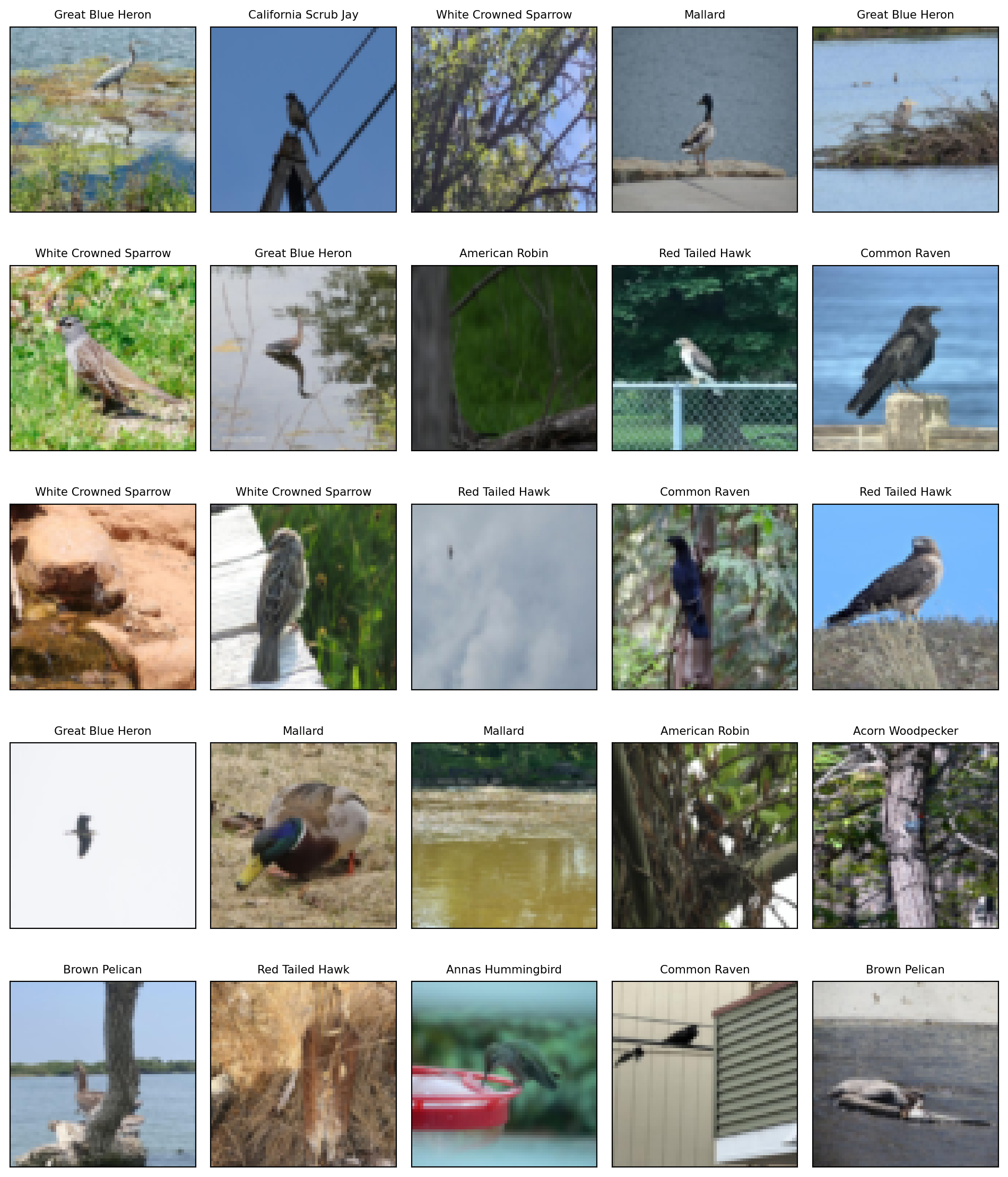
Before we start building the network, lets look at some sample images from the dataset. So that images look normal to us, we will reverse the normalization we performed earlier and store the results in bird_display.
Step 3: Specifying a Network: Classes and Inheritance
To fit the neural network, we first set up a model structure that describes the network. Doing so requires us to define new classes specific to the model we wish to fit. Typically this is done in PyTorch by sub-classing a generic representation of a network, nn.Module, which is the approach we take here.
Indented beneath the class statement are two methods: __init__ and forward. The __init__ method is called when an instance of the class is created. In the methods, self always refers to an instance of the class. In __init__, we attach objects to self as attributes; these are used in the forward method to describe the map that this module implements.
There is one additional line in __init__: a call to super(). This function allows subclasses to access methods of the class they inherit from. For torch models, we will always make this super() call, as it is necessary for the model to be properly interpreted by torch.
We specify a moderately-sized CNN, similar in structure to Figure 10.8 in the textbook. We use several layers, each consisting of convolution, ReLU, and max-pooling steps. We first define a module that defines one of these layers, a BuildingBlock.
Code
class BuildingBlock(nn.Module): # Define custom Neural Network moduledef__init__(self, in_channels, out_channels):super(BuildingBlock, self).__init__() # Initialize parent NN module# Padding='same' keeps spatial dimensions unchanged after convolutionself.conv = nn.Conv2d(in_channels=in_channels, out_channels=out_channels, kernel_size=(3, 3), # 3 x 3 filter padding='same') # Add padding so the input height and width match the output ( only depth changes)self.activation = nn.ReLU() # ReLU Activation function: zeros out negative values, allowing network to learn complex patternsself.pool = nn.MaxPool2d(kernel_size=(2, 2)) # Pooling layer that slides 2 x 2 window over the feature map and keeps only the largest value in each windowdef forward(self, x): # Defines data flow: Conv2D -> ReLU -> MaxPool2dreturnself.pool(self.activation(self.conv(x)))
Each BuildingBlock learns to detect visual features (edges, textures, color patterns) in its input, then uses max-pooling to shrink the image by half. After stacking three blocks, our 64×64 image has been compressed down to an 8×8 grid with 128 feature channels. We then flatten that into a single vector of 8,192 values and pass it through two fully-connected layers to produce a score for each of the 10 bird species.
Code
class BirdModel(nn.Module):def__init__(self):super(BirdModel, self).__init__()# Three blocks: channels grow 3→32→64→128; spatial dims shrink 64→32→16→8 sizes = [(3, 32), (32, 64), (64, 128)]self.conv = nn.Sequential(*[BuildingBlock(in_, out_) # x → BuildingBlock(3,32) → BuildingBlock(32,64) → BuildingBlock(64,128) → outputfor in_, out_ in sizes])self.output = nn.Sequential( nn.Dropout(0.5), # Randomly zeros out 50% of neurons during training to reduce overfitting nn.Linear(128*8*8, 512), # 128 feature maps of size 8×8 → 8,192 inputs nn.ReLU(), nn.Linear(512, 10) )def forward(self, x): val =self.conv(x) val = torch.flatten(val, start_dim=1)returnself.output(val)bird_model = BirdModel()
We can check that the model produces output of expected size by passing a batch through it, and use the summary() function to neatly display the shape and parameter count of each layer. We specify the size of the input and see the size of each tensor as it passes through the layers of the network.
Code
# Pass the same batch shape we saw earlier to verify output sizes at each layersummary(bird_model, input_size=X_.shape, col_names=['input_size', 'output_size', 'num_params'])
The summary() output is a layer-by-layer map of everything that happens to your data as it flows through the network. Here’s how to read it:
Columns
Input Shape — the tensor shape entering that layer (including the batch size of 32 as the first dimension)
Output Shape — the tensor shape leaving that layer
Param # — the number of learnable weights inside that layer
What the rows tell us
The indented tree mirrors how we built the model. Each BuildingBlock contains three sub-layers (Conv2d → ReLU → MaxPool2d), which are shown indented beneath it.
Conv2d — applies learned filters to detect visual features (edges, textures). Notice the spatial size stays the same after convolution (64→64, 32→32, etc.) because we used padding='same', but the number of channels grows (3→32→64→128) as the network learns increasingly complex features.
ReLU — a simple activation function; shapes don’t change.
MaxPool2d — this is where the spatial shrinking happens. Each block’s max-pool halves both height and width: 64→32→16→8. No parameters are learned here; it just summarizes the most active feature in each 2×2 patch.
Dropout — randomly zeros out neurons during training to prevent overfitting. No parameters; shapes don’t change.
Linear [32, 8192] → [32, 512] — after the three blocks, the 128 feature maps of size 8×8 are flattened into a single vector of 128×8×8 = 8,192 values, then mapped to 512. This is the largest layer: 8,192 × 512 = 4,194,816 parameters, which is ~97% of the entire model.
Linear [32, 512] → [32, 10] — the final layer produces one score per bird species. The class with the highest score is the model’s prediction.
Step 4: Training the Model
We use the RMSprop optimizer with a learning rate of 0.001. Experiments show that a smaller learning rate performs better than the default for image data. The optimizer takes the model’s parameters as its first argument, which informs it which values are involved in stochastic gradient descent (SGD).
SimpleModule.classification() wraps our BirdModel and automatically uses cross-entropy loss (the standard loss for multi-class classification) and tracks accuracy as a metric. CSVLogger records training and validation metrics to a CSV file after each epoch, which we will read back to plot training curves.
We define a summary_plot() helper (following the textbook) that plots training and validation curves for any logged metric over epochs. CSVLogger logs train and validation metrics at different steps, so the CSV contains NaN rows for each; dropna filters these before plotting.
Code
def summary_plot(results, ax, col='loss', valid_legend='Validation', training_legend='Training', ylabel='Loss', fontsize=20):# Training accuracy is logged as train_{col}_epoch; loss as train_{col} train_col = (f'train_{col}_epoch'iff'train_{col}_epoch'in results.columnselsef'train_{col}')for (column, color, label) inzip( [train_col, f'valid_{col}'], ['black', 'red'], [training_legend, valid_legend] ): results.dropna(subset=[column]).plot(x='epoch', y=column, label=label, marker='o', color=color, ax=ax) ax.set_xlabel('Epoch') ax.set_ylabel(ylabel)return ax
SimpleModule.classification() uses cross-entropy loss. We supply our RMSprop optimizer with a learning rate of 0.001 rather than the default, since experiments show it performs better on image data. The ErrorTracker callback records per-epoch metrics so we can inspect them after training.
GPU available: True (mps), used: True
TPU available: False, using: 0 TPU cores
IPU available: False, using: 0 IPUs
HPU available: False, using: 0 HPUs

  | Name  | Type             | Params
-------------------------------------------
0 | model | BirdModel        | 4.3 M
1 | loss  | CrossEntropyLoss | 0
-------------------------------------------
4.3 M     Trainable params
0         Non-trainable params
4.3 M     Total params
17.173    Total estimated model params size (MB)
`Trainer.fit` stopped: `max_epochs=30` reached.
Recall from Section 10.7 of the textbook that an epoch amounts to the number of SGD steps required to process all \(n\) training observations. Since our training set has 1,400 observations and we specified batch_size=32, an epoch corresponds to roughly \(1{,}400 / 32 \approx 44\) gradient steps.
Step 5: Evaluating the Model
After fitting, we read the logged metrics from the CSV file and plot training and validation curves. Then we evaluate final performance on the held-out test data using trainer.test(), which runs the model in evaluation mode.
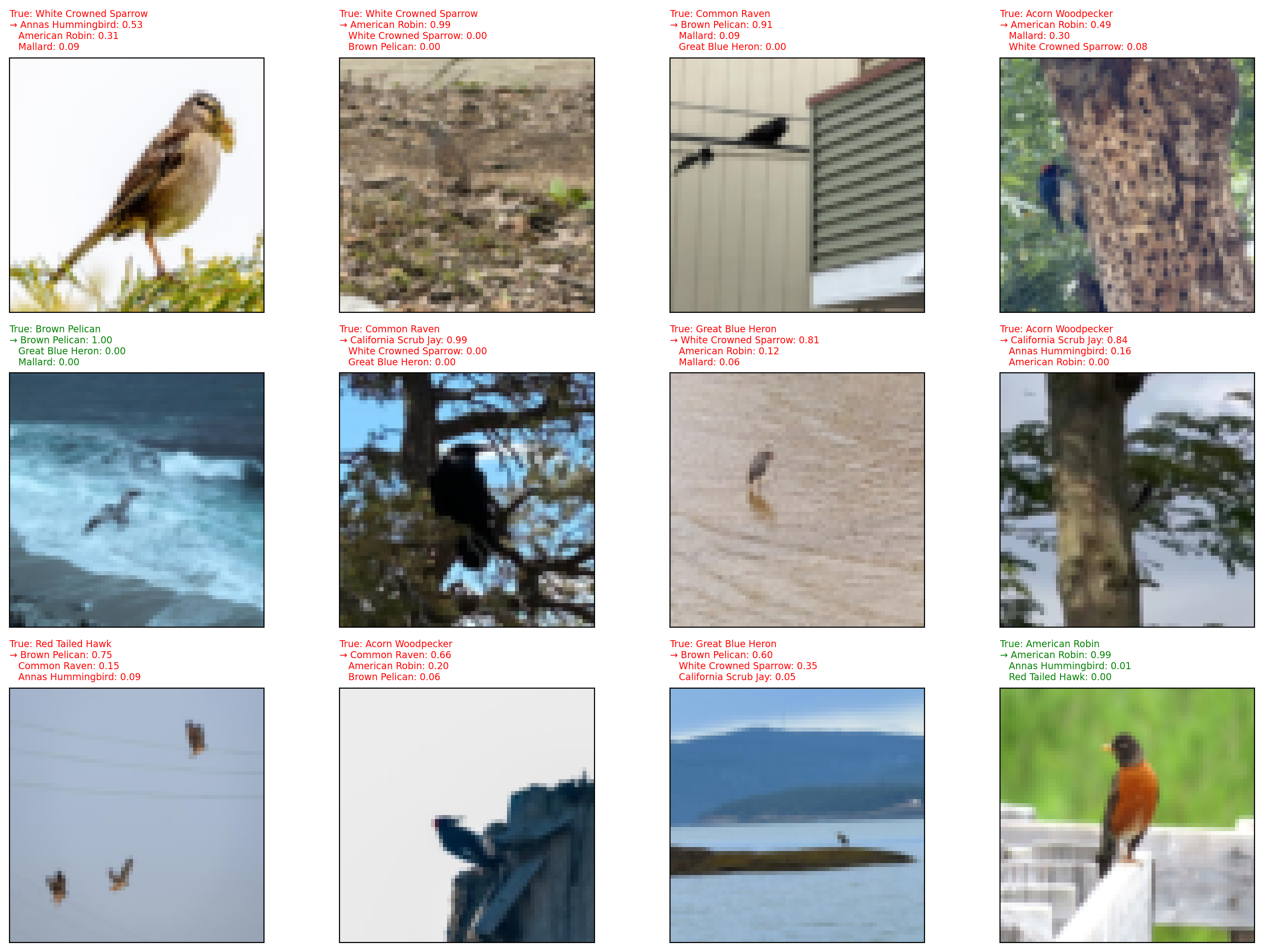
We can visualize what the model is actually doing by showing sample test images alongside its top-3 predicted species and their probabilities. The → marks the top prediction; titles are green if the model’s top prediction is correct and red if not. Probabilities come from applying softmax to the raw output scores, which converts them into values that sum to 1 across all 10 classes.
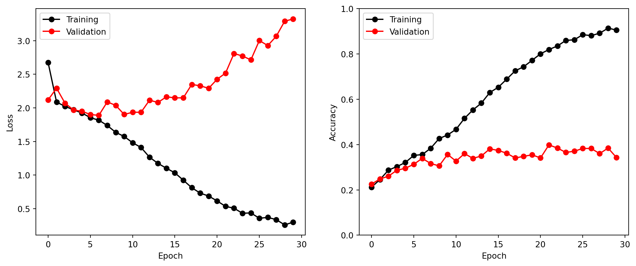
We now create plots of loss and accuracy as a function of the number of epochs. The training curve (black) reflects how well the model fits the training data. The validation curve (red) reflects generalization to unseen data. A growing gap between the two is the signature of overfitting, where the model is memorizing training examples rather than learning features that generalize to new images.
Code
bird_results = pd.read_csv(bird_logger.experiment.metrics_file_path)fig, axes = subplots(1, 2, figsize=(13, 5))# loss curves: a growing gap between training (black) and validation (red) signals overfittingax = summary_plot(bird_results, axes[0], col='loss', ylabel='Loss')ax.set_xticks(np.linspace(0, 30, 7).astype(int))# accuracy curvesax = summary_plot(bird_results, axes[1], col='accuracy', ylabel='Accuracy')ax.set_ylim([0, 1])ax.set_xticks(np.linspace(0, 30, 7).astype(int))
Cleanup
We delete the objects we created above to free memory.