End-to-End ML Workflows
EDS 232 · Machine Learning in Environmental Science
We will walk through the core steps of an end-to-end ML project:
- Framing the problem and understanding the big picture
- Getting the data and doing preliminary exploration
- Creating and locking away a test set
- Exploring and cleaning the training data
- Preparing data for ML (scrubbing, scaling, encoding)
- Trying candidate models and evaluating with CV
- Diagnosing what went wrong and going back to the drawing board
- Final model selection, tuning, and evaluation
The end-to-end workflow
. . .
- Understand the big picture
- Get the data and do a preliminary exploration
- Create a representative test set and lock it away
- Explore the train data to gain insights
- Consider attribute combinations
- Prepare train data for ML algorithms
- Try out different candidate models and estimate accuracy metrics with CV
- Go back to the drawing board if needed
- Select a model and fine-tune it
- Evaluate model on test set
🌟 Present your results!
Goals of this step:
- Identify any cleaning or transformations needed
- Identify promising predictors
- Brainstorm new features worth computing
For each variable, study:
- Type (categorical, int/float, bounded/unbounded)
- % of missing values
- Noisiness (outliers, rounding errors)
- Type of distribution
- Whether it is plausibly useful for the task
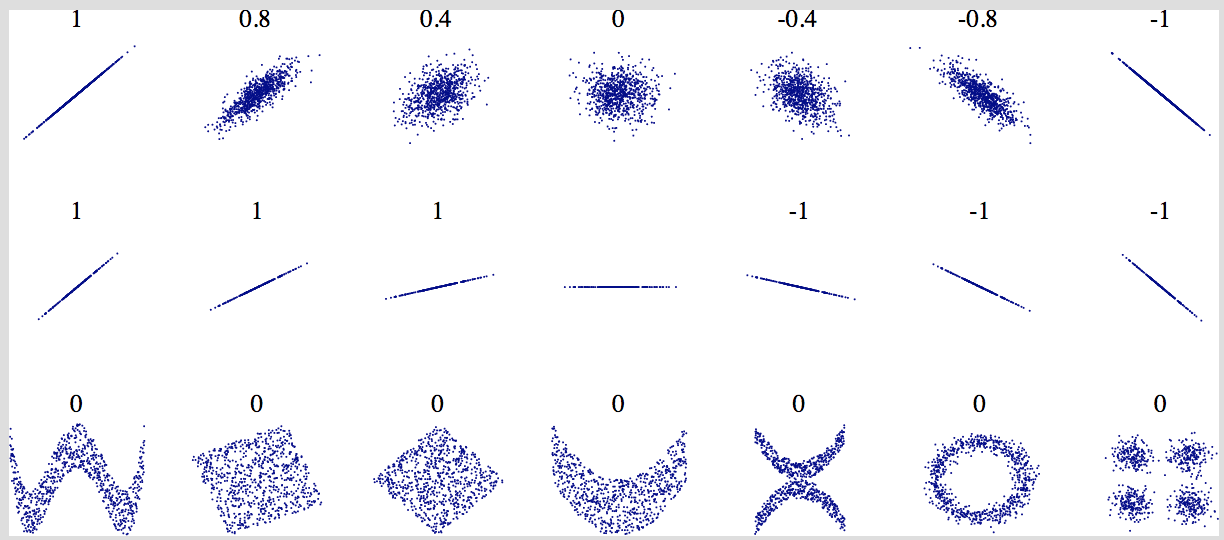
Plot each predictor against the target to uncover noise and correlations. Also compute pairwise correlations using .corr().
Important: .corr() only works for numerical variables and only measures linear association.
- Close to +1 → strong positive linear correlation
- Close to –1 → strong negative linear correlation
- Close to 0 → no linear correlation (but a non-linear relationship may still exist!)
Sometimes combining predictors produces a more informative feature than either one alone.
- Whenever possible, ground decisions in domain expertise
- This is an iterative process — revisit as the model develops
Preparing data for ML
High-quality training data is critical. Common issues:
- Omitted values (missing data)
- Duplicate observations
- Outliers
Potential fixes for each:
| Approach | When to use |
|---|---|
| Remove the observation | Missingness is random and n is large |
| Impute (mean, median, KNN…) | Losing observations is costly |
| Drop the entire feature | Variable has too many missing values or is not useful |
Always keep a backup of the raw data before transforming!
Many ML models perform better when features are on similar scales.
Standardization (StandardScaler): subtract the mean, divide by the standard deviation → zero mean, unit variance.
The target variable does not need to be scaled.
Linear scaling, clipping, and log-scaling are a few other ways you may want to scale your data. You can read a brief overview about each here.
Applied to categorical predictors.
Suppose you have a variable called biome with categories savanna, rainforest, grassland, and desert.
Most ML algorithms prefer to work with numerical variables, so we can transform this variable into numbers.
. . .
An easy way would be to assign each with a number:
savanna-> 0rainforest-> 1grassland-> 2desert-> 3
. . .
One issue with this approach is that a model would treat the consecutive numbers as a numerical variable that contains information about the relative order between them.
One-hot encoding creates a binary feature per class:
- new feature equals 1 when the observation belongs to the class,
- new feature equals 0 if the observation does not belong to the class.
. . .
For example, the one-hot encoding for the biome classes would look like:
| Observation | savanna |
rainforest |
grassland |
desert |
|---|---|---|---|---|
| biome = savanna | 1 | 0 | 0 | 0 |
| biome = rainforest | 0 | 1 | 0 | 0 |
| biome = grassland | 0 | 0 | 1 | 0 |
| biome = desert | 0 | 0 | 0 | 1 |
Each row has exactly one 1 and all other values 0.
. . .
For linear models, drop one encoded column to avoid perfect multicollinearity (drop parameter in OneHotEncoder).
Once you have a solid, clean training set:
- Select a few candidate models appropriate for the problem setup
- Train with default hyperparameters — don’t over-invest yet
- Estimate performance with cross-validation (or ROC curves for classification)
The goal is a quick, comparable baseline across model families. Tuning comes later.
Evaluating and refining
If, at this point, your results are bad, there are generally two things that could have gone wrong: “bad model” or “bad data”.
| Problem | Description | Fix |
|---|---|---|
| Too small | More high-quality data generally helps | Collect more data |
| Nonrepresentative | Sampling noise or bias | Better sampling strategy |
| Poor quality | Outliers, errors, missing values obscure signal | Drop, correct, or impute |
| Irrelevant features | Noise prevents the algorithm from finding signal | Feature selection or extraction |
| Problem | Description | Fix |
|---|---|---|
| Overfitting | Model memorizes training noise; poor generalization | Simpler model; more data; reduce variance via hyperparameters |
| Underfitting | Model too simple to capture data structure | More flexible model; more informative features |
. . .
Whatever the challenge: it’s ok to go back and experiment with different feature combinations and models.
9. Fine-tune the selected model.
Use cross-validation on the training set to search over hyperparameter combinations (e.g., GridSearchCV). All tuning decisions must use training data only — the test set stays locked!
. . .
10. Evaluate on the test set.
Evaluate exactly once. If test performance is much worse than your CV estimate, the model likely overfit during tuning.
. . .
🌟 Present your results.
Report the metric value and its practical meaning. Document the full pipeline, decisions made at each step, and any caveats about where the model may not generalize.